Aquatic ecosystem assessments for rivers
Information for assessing riverine ecosystems and identifying changes to those systems from instream developments.
Aquatic Research Series 2013-06
Robert A. Metcalfe, Robert W. Mackereth, Brian Grantham, Nicholas Jones, Richard S. Pyrce, Tim Haxton, James J. Luce, Ryan Stainton
November 2013
© 2013, Queen’s Printer for Ontario
ISBN 978-1-4606-3215-4 (PDF)
This publication was produced by:
Aquatic Research and Monitoring Section
Ontario Ministry of Natural Resources
2140 East Bank Drive
Peterborough, Ontario
K9J 8M5
This document is for scientific research purposes and does not represent the policy or opinion of the Government of Ontario.
This technical report should be cited as follows:
Metcalfe, R.A., Mackereth, R.W., Grantham, B., Jones, N., Pyrce, R.S., Haxton, T., Luce, J.J., Stainton, R., 2013. Aquatic Ecosystem Assessments for Rivers. Science and Research Branch, Ministry of Natural Resources, Peterborough, Ontario. 210 pp.
Cette publication hautement spécialisée Aquatic Ecosystem Assessments for Rivers n’est disponible qu’en anglais en vertu du Règlement 411/97, qui en exempte l’application de la Loi sur les services en français. Pour obtenir de l’aide en français, veuillez communiquer avec le ministère des Richesses naturelles au NRISC@ontario.ca.
Foreword
This document is intended to provide information for assessing the current state of riverine ecosystems and identifying potential changes to those systems resulting from in- stream development (including re-developments and operational changes). The framework and approach may also be applied to other factors causing the alteration of river processes (e.g. climate and land use changes). The ecosystem assessment indicators described in this report are ecological measures, not social or economic considerations.
Acknowledgements
Development of the assessment framework benefited from the contributions of Trevor Friesen, Steve McGovern, Mark Sobchuk, Sandra Dosser, Emily Hawkins, Fiona McGuiness, and Audie Skinner. Also acknowledged are those who were involved in earlier discussions that framed the evolution of this document including the Institute for Watershed Science, Trent University and the many people who provided comments and suggestions on earlier drafts.
Executive summary
Aquatic Ecosystem Assessments for Rivers (AEAR) provides a science-based framework for assessing the ecological condition of river ecosystems, the state of valued ecosystem components (VECs) within rivers and the changes expected to arise in response to in-stream development. The assessment framework is designed to provide technical information on a standardised approach for assessing the current state of riverine ecosystems and identifying potential changes to riverine ecosystems resulting from the alteration of physical and biological processes. Although the document often uses the construction and operations of dams as an example, the framework and approach can be applied to any in-stream development or other factors (e.g. climate and land-use changes) that may alter water levels and flows in a riverine environment.
The assessment framework was developed based on the following guiding principles: that it provides a science-based approach, provides technical information that is flexible to varying scales of development, and is consistent and transparent in its application. It is grounded in ecological concepts of ecological condition and ecological integrity as the basis to assess and describe the current state and degree of alteration in river ecosystems, river system connectivity, the range of natural variability in river ecosystems, and the relationship between ecological condition and system alteration. The assessment framework provides a step-by- step process for practitioners to identify the zone of influence for a project, implement a sampling design to characterise the current ecosystem state and establish a reference condition, assess the degree of alteration and identify opportunities for mitigation, predict the effect of the remaining alteration on biological indicators and ecological condition, and to conduct post-alteration monitoring.
Aquatic Ecosystem Assessments for Rivers identifies key ecosystem components that have important functions in determining the integrity of river ecosystems. These include the hydrologic regime, sediment regime, water quality, thermal regime, and biologic components. For each ecosystem component, a series of indicator variables are identified which are thought to best represent, or be important determinants of, ecosystem integrity. Indicator variables are intended to provide sufficient information to characterize a river ecosystem, evaluate its ecological condition and the state of VECs. Alteration of riverine processes as a result of in-stream development or other factors are assessed based on the expected changes in physical and chemical indicator variables relative to their existing or natural state. Where possible, changes in an indicator variable are assessed using criteria based on the expected magnitude of deviation from a natural reference condition and categorized as being low, medium, or high alteration. Based on an overall assessment of predicted changes in physical and chemical indicator variables, expected responses in the biological indicator variables are determined and potential changes in the ecological condition of the river ecosystem or state of VECs, predicted. Understanding the natural range of variability in indicator variables in river ecosystems and the relationship between ecological condition and system alteration are fundamental concepts underlying the framework. This understanding increases certainty in predicting the effects of an alteration and interpreting changes in indicator variables following an alteration.
Chapter 1: The aquatic ecosystem assessment framework
1.0 Introduction
Fresh water lakes and rivers contain less than 1% of the world’s water supply but are responsible for supporting significant biodiversity in both terrestrial and aquatic ecosystems and providing a range of services important for human health and well-being as well as social and economic benefits. Fresh water in these ecosystems is a finite resource for which there is increasing demand caused by a combination of population growth, increased consumption, and a changing climate. The ability to assess the condition of lake and river ecosystems, evaluate sensitivity to alteration, and identify potential changes to the ecosystem resulting from different development and re- development options is important to inform decision making. This document provides an assessment framework and technical information for assessing potential changes to aquatic ecosystems arising from in-stream development or other factors. Although the document often uses the construction and operations of dams as an example, the framework and approach can be applied to any in-stream development or other factors (e.g. climate and land use change) that may alter water levels and flows in a riverine environment.
The aquatic ecosystem assessment framework serves at least two purposes:
- Assist practitioners in assessing how alteration to a river’s characteristics may affect aquatic ecosystem health at a local development site. This assessment will inform a decision-making process and the implementation of a post-alteration monitoring program; and
- Build knowledge that can inform future policy and management directions by allowing the analysis of information collected in a standard way across sites consistent with an adaptive management approach.
The content of this document focuses on aquatic ecosystem processes in rivers and includes information on reservoirs only to the extent where it is important for understanding the alteration to downstream riverine processes. It is recognised, however, that a similar effort is needed to assess the effects of altering water level regimes on ecological condition and valued ecosystem components (VECs) of reservoirs.
2.0 Guiding principles
The following principles were followed to ensure this document informs application review, construction, redevelopment, and operation of in-stream developments:
- Develop a practical science-based approach to assess the potential effects of in- stream development or other factors on aquatic ecosystems;
- Develop technical information that is flexible to varying spatial and temporal scales and development structures and operations; and
- Develop a framework that is consistent and transparent in its application.
In addition to the guiding principles above, the scientific approach in this document has been developed with the intent that the associated work will, to the fullest extent possible:
- Maximize the value on science investment to both MNR and developers;
- Contribute to a better understanding of the effects of different in-stream developments and other factors on river ecosystems;
- Provide proponents with high quality background data to support future project planning, environmental assessments, and project development and operation;
- Support an adaptive management approach that leads to ongoing improvements in facility design, operation, and mitigation techniques, inform future policy development and application approval processes, and ultimately, to better management of Ontario’s aquatic ecosystems.
An important objective of the approach presented in this document is to encourage the use of common indicators and data collection methods. Doing so will provide improved clarity to MNR staff and proponents on the process and information required to conduct aquatic ecosystem assessments. It will also provide the opportunity to learn from the collective information to support policy development and management decision making in the future consistent with an adaptive management approach. Using these data collection and assessment methodologies also provides comparable and consistent information necessary to assess cumulative effects on a river system.
3.0 The assessment framework
Assessing system alteration associated with a proposed development and predicting and monitoring changes to river ecosystems is accomplished using a standardized assessment framework to characterize the physical, chemical and biological components of the ecosystem. These components are characterized using a series of indicator variables (i.e. quantitative or qualitative variables which are representative of the ecosystem). The extent to which indicator variables are expected, or observed, to change in response to in-stream development or other factors form the basis for evaluating the change to the aquatic system’s ecological condition. The ecological concepts underlying the assessment framework are described in Appendix 1.
This assessment framework is designed to help address the following questions:
- What does the system look like now (physically, chemically, biologically)?
- If already altered, what did the system look like before it was altered?
- What is the planned development (including its operation)?
- How are the physical, chemical and biological components expected to change after the planned development and what is the expected effect on ecological condition?
- Can change be prevented and/or mitigated if necessary? If yes, re-evaluate expected changes.
- What is the system expected to look like after the alteration and mitigation?
- What monitoring would be most appropriate for assessing post-alteration ecological condition?
This assessment framework may then serve as input into a decision-making process, including a risk assessment, which includes similar information about social and economic values.
3.1 Relating ecological condition to system alteration
Alterations to ecosystems, either by natural or anthropogenic processes, are expected to have some effect on their ecological condition. A conceptual model commonly used to relate system alteration to ecological condition is shown in Figure 1. Ecological condition is a qualitative summary of the state of an ecosystem relative to its natural condition. System alteration is a change to any ecosystem characteristic resulting from a perturbation. The nature of the relationship between alteration and ecological condition, shown as the ecological response, is complex and will depend on the type of alteration, as well as the sensitivity and resilience of the ecosystem. For simplicity, a linear relationship is shown in Figure 1; although, in most cases, the relationship would likely be non-linear (e.g. ecological condition changing abruptly at some threshold level of alteration).
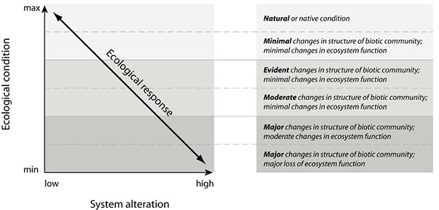
System alteration, illustrated on the x-axis of Figure 1, corresponds to the magnitude of alteration to an ecosystem’s characteristics relative to its natural condition. Where multiple alterations have occurred, this point represents the cumulative alteration to the ecosystem. Ecological condition, illustrated on the y-axis 1, is a qualitative summary of the state of an ecosystem. Points along the y-axis correspond to the degree of change in ecosystem structure and function, and hence, ecosystem integrity (see appendix 1), resulting from system alterations. Ecological condition is assumed to be at its maximum in unaltered ecosystems and at a minimum in ecosystems that have experienced high levels of alteration.
Quantifying alteration, ecological condition, and the relationship between them is challenging due to the complexity of ecosystem functions and responses that are often non-linear and likely vary among systems. As a result, a more simplified approach is often used which describes the relationship between alteration and ecological condition as a series of qualitative categories (Figure 1). While it is unlikely that a single alteration event would shift ecological condition across the entire range of categories, a number of independent alterations to a system can have cumulative effects on the ecological condition.
This conceptual model underpins the assessment framework described in this document to address the questions listed in Section 3.0. It provides the basis for relating system alteration resulting from an in-stream development to potential changes to ecosystem condition. In this case, system alteration is a combination of the direct effects of the in-in- stream development, as well as its operation on the physical and chemical characteristics of the ecosystem. These could include changes to the hydrologic, sediment, thermal and water quality characteristics of the river system, which in turn may affect its biological characteristics. The assessment framework identifies a suite of individual indicator metrics, the state of which can be measured/predicted and compared to their expected range of indicator values in a reference system (e.g. natural). Taken together, the indicators form the basis for characterizing the magnitude of an alteration which in turn is used to predict a potential change in ecological condition. The assessment framework does not quantify alteration and ecological condition, but rather categorizes alteration as being low, medium, and high and ecological condition using the descriptions in Figure 1.
This assessment framework offers no guidance on what constitutes an acceptable amount of change from either the natural or current condition. Its purpose is simply to provide a basis for evaluating how system alterations may relate to changes in ecosystem condition.
This approach of characterizing system alteration and ecosystem condition as categories, based on a comparison to a natural condition is not unique. There are numerous examples around the world where natural reference conditions and measures of ecological condition are used to assess river health. Natural reference conditions have been used to support implementation of the Clean Water Act in the United States, the Water Framework Directive in the European Union, South Africa’s National Water Act (DWAF 1999), and the Australian River Assessment System (AUSRIVAS), a rapid prediction system used to assess the biological health of Australian rivers. The reference condition approach is also the basis for the Canadian Aquatic Biomonitoring Network (CABIN), an aquatic biological monitoring program for assessing the health of freshwater ecosystems in Canada. Regional assessments of the relationships between ecological condition and alteration from a natural reference condition are also receiving increased attention (e.g. Carisle et al. 2010).
3.2 Ecological characterization: Identifying key ecosystem components
The ecological condition of an aquatic ecosystem is the result of a complex, interdependent set of physical, chemical and biological elements. Thus, characterising the system can be facilitated by evaluating key ecosystem components which have important functions in determining ecosystem integrity. These include biological components and hydrologic, sediment, water quality and thermal regimes, along with their associated connectivity and variability.
3.2.1 Biological components
All development activities that alter the hydrologic and water quality characteristics of a river have some degree of effect on riverine biota and their habitat. These will typically occur at multiple trophic levels. For example, game fish species are valued ecosystem components (VECs) within rivers and maintaining their populations is often a primary concern for social and economic reasons. However, fish communities depend on the function of all lower trophic levels, so they can serve as an overall reflection of the health of the river ecosystem (Poff et al. 1997). Primary production supports higher trophic levels as a food source (e.g. periphyton) and can provide physical habitat in the form of aquatic macrophytes and riparian vegetation. All these ecosystem components can be affected by alteration to the hydrological, sediment, water quality, and temperature regime, so it is important that numerous indicators, including all trophic levels, be measured as part of a site characterization and monitoring plan.
3.2.2 Hydrologic regime
Flow is the dominant variable determining the form and function of a river. Flow alteration changes the pattern of natural variation and disturbance on a river system. Depending upon the type of in-stream development, this may include converting the river to a lake-like (lentic) ecosystem upstream of the project and modifying the natural flow regime (magnitude, duration, frequency, timing, and rate of change) downstream of the project. Such changes may propagate extensive distances downstream depending on the degree of alteration and river morphology. Understanding the ecological functions provided by the natural flow components is necessary for assessing the potential alteration to ecological condition and VECs.
3.2.3 Sediment regime
Natural rivers have highly variable processes of erosion, transport, and deposition of suspended sediment and bedload sediment that are intricately tied to changes in water velocity, sediment supply and shape, channel slope, and the roughness of channel material. The result is a dynamically changing channel form that produces a diversity of physical habitat important for maintaining ecological integrity. Structures, such as dams, act as sediment traps, interrupting the longitudinal connectivity of the sediment regime, resulting in decreased downstream turbidity and sediment load that may lead to armouring of channels and increased erosion as the system attempts to rebalance itself. Moreover, reductions in peak flows during freshet can reduce the river’s ability to transport materials deposited in the main river by tributaries, potentially resulting in the formation of deltas and other changes in river morphology. Changes in the sediment regime can result in changes to quality, quantity and distribution of habitat for biological components of aquatic ecosystems. In addition, there can be changes in migration and movement patterns and productivity of the system.
3.2.4 Water quality and thermal regimes
A river’s water quality, including the temperature regime, is influenced by a variety of factors, including climate, the geological characteristics of the drainage basin, flow regime, and other factors such as land use patterns. For example, a significant change in the flow regime or creation of a reservoir can alter water temperatures, dissolved gases, nutrients, turbidity/light, and the bio-availability of contaminants within a river. Such changes can affect all trophic levels.
Water temperatures limit and/or determine the distribution and abundance of many riverine species. Temperature influences overall water quality, rates of nutrient turnover, metabolic activity and growth rates, timing of migration and spawning events and the distribution of stream organisms. Hence, a river’s thermal regime strongly influences ecological condition. Species-specific thermal preferences and tolerances are critical biological characteristics that define thermal habitat. For example, the conversion of rivers to lake-like ecosystems upstream of dams can alter the thermal regime upwards of 930 km downstream (Olden and Naiman 2010). Depending on the design of the dam, downstream water temperatures may decrease if water is drawn from the cold hypolimnion or increase if water is drawn from the warm epilimnion. Such fundamental changes to the thermal regime and their potential consequence on aquatic ecosystems, are frequently overlooked, yet are some of the more easily mitigated issues when considering new and, in some cases, existing development.
3.3 Indicators
Indicators for the key ecosystem components described in the previous section are summarised in Table 1 and detailed in subsequent chapters. Indicators for physical and chemical components cover a range of processes and functions thought to be the primary determinants of change in the biologic indicators. These include flow, sediment movement, water temperature, and dissolved oxygen. Biologic indicators include a variety of measures to assess the structure and function of an ecosystem.
Together, the indicators in Table 1 can be used to assess the current state of the aquatic ecosystem and evaluate its ecological condition. However, not all of the indicators are appropriate for every project. The choice of indicators will be part of the decision process for a specific project and will be based on the type of alteration and the characteristics of the site. Additional indicators may also be considered to facilitate comparisons at other sites and to assess cumulative effects. It is also important to keep in mind that multiple indicators can often be sampled using the same method (e.g. water quality, temperature).
| Key ecosystem component | Characteristic | Indicator |
|---|---|---|
| Hydrologic regime | Baseflow | Monthly median baseflow magnitude. |
| Hydrologic regime | Subsistence flow | Monthly 95% exceedance flow magnitude of total streamflow |
| Hydrologic regime | Subsistence flow | % wetted perimeter |
| Hydrologic regime | High flow pulses < bankfull | Monthly median frequency and duration (days) of flow events less than the bankfull flow magnitude |
| Hydrologic regime | Channel forming flow | Magnitude, duration and timing of flows with a recurrence interval of 1.5 years |
| Hydrologic regime | Riparian flow | Magnitude, duration and timing of flows with recurrence intervals of 2, 10, and 20 years |
| Hydrologic regime | Rate of change of flow | Monthly median rate-of-change of flow for rising and falling limbs of flow events |
| Sediment regime | Sediment transport – Suspended | Mean annual suspended sediment yield |
| Sediment regime | Sediment transport – Bedload | Annual bankfull flow duration |
| Sediment regime | Sediment transport – Bedload | Annual excess shear power |
| Sediment regime | Channel form and habitat | Sinuosity index |
| Sediment regime | Channel form and habitat | Mean width-depth ratio |
| Sediment regime | Channel form and habitat | Bed composition |
| Water quality | Dissolved gases | Dissolved oxygen concentration |
| Water quality | Dissolved gases | Total dissolved gases |
| Water quality | pH | pH |
| Water quality | Alkalinity | Alkalinity |
| Water quality | Conductance | Specific conductance |
| Water quality | Dissolved solids | Total dissolved solids |
| Water quality | Suspended solids | Total suspended solids |
| Water quality | Turbidity/light transmission | Nephelometric Turbidity (NTUs) |
| Water quality | Turbidity/light transmission | Secchi disk depth |
| Water quality | Nutrients | Total Phosphorus |
| Water quality | Nutrients | Total Kjeldahl Nitrogen |
| Water quality | Nutrients | Nitrate/Nitrite |
| Water quality | Nutrients | Total Ammonia |
| Water quality | Organic matter | Dissolved Organic Carbon |
| Water quality | Primary productivity | Chlorophyll-a |
| Thermal regime | Guild | Summer thermal class (June, July and August) |
| Thermal regime | Timing | Mean annual date of maxima and minima |
| Thermal regime | Timing | Monthly modal hour of daily maxima and minima |
| Thermal regime | Magnitude | Mean annual maxima and minima |
| Thermal regime | Magnitude | Monthly means of daily maxima and minima |
| Thermal regime | Variability | Mean annual temperature range |
| Thermal regime | Variability | Monthly means of daily temperature range |
| Thermal regime | Rate of change | Monthly means of daily maximum hourly rates of change (positive and negative) |
| Thermal regime | Duration | Species specific temperature duration ±2 °C of preferred temperatures and ≥ lethal temperatures during the summer period |
| Biology | Fish | Fish presence and absence |
| Biology | Fish | Fish community composition |
| Biology | Fish | Index of abundance for VECs |
| Biology | Fish | Size structure |
| Biology | Fish | Young of year (YOY) index of abundance |
| Biology | Fish | YOY growth |
| Biology | Fish | Methyl mercury in fish tissue |
| Biology | Benthos | Composition and abundance of dominant invertebrates |
| Biology | Benthos | Percentage Anisoptera Plecoptera Trichoptera Ephemeroptera |
| Biology | Basal resources | Biomass of coarse particulate organic matter |
| Biology | Basal resources | Periphyton: Biomass of attached algae |
| Biology | Basal resources | Coverage of aquatic macrophytes |
For the purposes of this document, an indicator is defined as:
Indicators are intended to provide sufficient information to characterize components of an aquatic ecosystem prior to a development, redevelopment, or operational changes. Tracking the magnitude and direction of indicators over time provides a basis for evaluating the effectiveness of mitigation strategies, operating plans, and other management approaches for maintaining an accepted ecological condition or VEC state (i.e. effectiveness monitoring).
If the state of selected indicators changes significantly following construction or operational changes, the likelihood of a change in ecological condition or VEC state increases and more detailed evaluation of some ecosystem components may be necessary to determine the causal linkages between the alteration and ecosystem response (i.e. effects monitoring). Detailed studies of particular ecosystem components may also be required to evaluate potential effects on species of particular concern or their habitat (e.g. species at risk). Results of further studies can be used to assist in the development and implementation of adaptive management strategies.
3.4 Establishing a reference condition
A natural reference condition may be used to determine the state and natural range of variability of an indicator and to interpret the magnitude of changes in indicator values.
Riverine systems are naturally dynamic and any indicators measured will be highly variable, both spatially and temporally. A reference condition provides an estimate of the natural range of variability for an indicator which is necessary for interpreting changes in indicators following alteration. It also provides a baseline for assessing cumulative effects. Reference conditions can be obtained from: a) reference sites; b) historical knowledge; and/or c) modeling (see below).
In some instances, the reference condition for an indicator variable will not be known. As a result, changes in an indicator variable in response to an alteration are estimated based on knowledge of the current condition and the proposed alteration. There might also be uncertainty in the functional relationship between the degree of alteration and an indicator variable (see Figure 1). In these cases, we may not know when a threshold is being approached; a point where even a small alteration may result in significant changes to ecological condition or a VEC. Thus, confidence in predicting these changes will be greatest when the reference condition and functional relationship are known.
In this assessment framework a natural reference condition is used for the physical and chemical indicator variables, where possible, to assess the magnitude and direction of alteration to the system (see the x-axis in Figure 1). The physical and chemical indicator variables provide the basis for predicting potential change to ecological condition or VEC state. Establishing a natural reference condition for biological variables may also be possible, particularly if the current condition of a site is natural.
A natural reference system, (e.g. a similar unaltered river or upstream river reach) if monitored concurrently post alteration, can be used to determine whether changes in indicator values are related to natural variability in the system (e.g. drying conditions in the region) or changes associated with an alteration. The ability to differentiate between natural variability and the effects of alteration is important for evaluating the effectiveness of mitigation strategies.
Ideally, the reference condition will reflect the natural state of the ecosystem. However, in some regions of Ontario it may be difficult to determine what the natural state would have been since there are few unaltered rivers to serve as references. In this case, the natural reference condition may be represented by the “least disturbed reference condition”, as determined from the least impaired ecosystems with similar physical, chemical, and biological attributes. Thus, the reference condition for an indicator would be the ‘typical’ conditions observed in the absence of any anthropogenic stressor, or the least number of stressors.
There are several approaches for defining a reference condition depending on the indicator(s) being assessed and the information available for a particular site:
- Reference Sites - A natural reference condition can be established by measuring indicators at a number of natural or least disturbed reference sites or at the same site for a long period of time. Reference sites may include existing monitoring sites or information could come from a database of comparable systems;
- Historical Information - Reconstruction of information from historical knowledge at the proposal site (e.g. traditional ecological knowledge - TEK); and/or
- Modeling - Modelling conditions for the development site using:
- Information from nearby sites (e.g. the simulation of historical natural flow regimes).
- Information from nearby sites to predict ecological attributes expected at a site from a suite of measured environmental variables.
3.5 Assessment criteria
For each indicator variable, the change, or ‘distance away’, from the reference condition is estimated using assessment criteria.
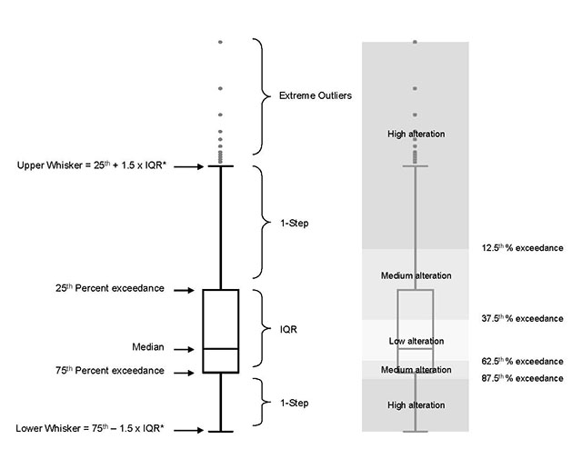
The natural range of variability observed in indicator variables is used to establish assessment criteria to evaluate the degree of expected or observed alteration, denoted simply as low, medium, or high alteration. The degree of alteration can be defined quantitatively when appropriate data are available or qualitatively when they are not. Quantitative values for assessment criteria will depend on the data available to establish the reference condition. When the number of observations of an indicator variable are sufficient to describe an underlying distribution, standard statistical methods for estimating measures of central tendency and dispersion are used to derive assessment criteria values For data that follows a normal distribution, the mean is used to estimate the most commonly observed values and standard deviations to describe the distance away from the mean. In this case, an alteration that resulted in an indicator variable remaining within one standard deviation of the reference condition (i.e. in the same range as 66% of all observations in the distribution) would be considered low alteration, within two standard deviations (i.e. within the distribution) medium alteration, and beyond two standard deviations (i.e. outside the distribution) high alteration. For data that does not follow a normal distribution (e.g. when extreme values are more common) the median is used to estimate the most commonly observed conditions and percentiles to provide measures of dispersion. The percentile criteria used to evaluate whether a change in the median of the indicator variable would be considered low, medium, or high alteration (for an example, see Figure 3 in Chapter 2: Hydrologic Regime).
4.0 Implementation
The basic process for implementing the framework described above is illustrated in Figure 2.
Figure 2: Schematic diagram of the process of assessing the level of alteration resulting from in-stream development, predicting the potential changes to ecological condition of the river system and monitoring the ecological condition following alteration
- The basic process for implementing the framework
- Step 1: Obtain information on the planned development
- Step 2: Identify the zone of influence
- Step 3: Characterise the current state of the ecosystem and establish the reference condition
- Are there site specific concerns that need to be addressed? (e.g. species at risk, DFO-HADD)
- Step 4: Assess the alteration
- i) Physical
- ii) Chemical
- iii) passage
- iv) Habitat
- Step 5: Predict the effect on the biological indicators
- Step 6: Is it necessary and possible to prevent/mitigate alterations?
- Yes? Return to Step 4
- No? Proceed to Step 7
- Step 7: Examine suite of indicators to predict chanes in ecological condition
- Input to decision making (e.g. approvals, adaptive management).
- Step 8: Post alteration monitoring
- Input to decision making (e.g. approvals, adaptive management).
4.1 Information on the planned development
A clear understanding of the proposed development (e.g. dam design, foot print location, operating regime) is needed to assess the degree of alteration expected. For example, in the case of dam construction and operation possible questions might include:
- Will the development impinge on any important habitat features?
- At what depth is the intake?
- Will the dam have sluice gates to flush sediment and nutrients?
- Will the turbines, if part of the development, be capable of passing lower flows?
- How will the dam be operated - daily, seasonally, and annually? What will be the reservoir morphology?
- What will be the residence time of the reservoir? Will there be a capability for passing fish?
- Will there be a diversion of water around a reach of the natural channel?
4.2 Identifying the zone of influence
The extent to which an in-stream development affects the physical, chemical, and biological characteristics of an ecosystem is called the zone of influence (ZOI). The spatial extent of the ZOI depends largely on the development’s location, design, and operation, how likely it is to be a barrier, and creation of reservoirs. The ZOI extends to where the alterations in physical, chemical, and biological processes are not discernible from natural variability. Generally, the zone of influence will increase in size as the degree of alteration and the size of the river increases. For example, a large waterpower peaking facility with a hypolimnetic draw may have an extensive ZOI compared to a small run-of-the-river facility. Olden and Naiman (2010) noted that recovery of thermal regime may require 40 to 930 km depending on characteristics of the dam and downstream reaches, lakes, groundwater inputs, and tributaries. Annual variation in weather conditions can also influence the extent of the ZOI.
Quantitative models can be used to predict the zone of influence based on a development’s design and operation. Many of these models require knowledge of physical and chemical processes e.g. flow and thermal regime, to generate predictions about the ZOI. While such knowledge can be gained through field data collection, this procedure would lengthen the time required for pre-alteration evaluation. Lewis et al. (2005) suggested that the ZOI extends downstream to a point on the river where the watershed area is five times larger than the watershed area draining to a waterpower site - essentially one part regulated flow to four parts natural flow. This attenuation is assumed to be sufficient to mask the altered physical and chemical regimes. Using this approach, the ZOI can be estimated by examining watershed areas. The watershed area approach is intended as a coarse rule of thumb to provide an initial estimate of the potential downstream ZOI and may be refined using site specific information.
The ZOI estimate may be further refined to include upstream sections of river. The hydraulic properties of the river are altered in the backwater zone upstream of a reservoir, being most pronounced closest to the dam. The upstream effect increases with impoundment elevation. Samuels (1989) provides a first order approximation of the upstream backwater extent based on the river slope and bankfull depth. In many cases the downstream hydraulic alteration of one reservoir overlaps with the upstream backwater effects of a downstream water body (e.g. dam or lake).
The upstream ZOI delineation may also consider the potential for the in-stream development to block fish movement. In some cases, a dam will be located at an existing waterfall or rapids that may or may not block passage. Fish migrate through river networks to access spawning habitat, over-wintering habitat, thermal refugia, and feeding areas (Northcote 1978). Maintaining these migratory pathways is important for the sustainability of fish and mussel populations.
4.3 Characterising the current ecosystem state
The most important part of this framework is to establish the current condition of the ecosystem. This will provide important baseline information from which all subsequent post-alteration monitoring will be compared. Estimating the full set of key ecosystem component indicators will obviously provide the most complete description of the current ecological condition or state of VECs at a site and provide the basis for a long-term monitoring program. However, this assessment framework is not meant to limit what is measured or how specifically the ecosystem is characterised. Those indicators identified are thought to provide a minimum standard suite necessary to establish a baseline ecosystem description, the current degree of alteration, and to assess change through long-term monitoring. In practice, a subset of indicators might be better suited to site specific conditions. In addition to the indicators listed, any other information available that builds knowledge of the system and informs the assessment process may be considered. This includes the use of traditional ecological knowledge of the historical and present day characteristics of the river ecosystem.
For systems previously altered, the current degree of alteration in each indicator variable is determined using assessment criteria based on the reference condition (i.e. low, medium, and high). In the absence of a reference condition for an indicator variable, the current degree of alteration will be unknown. In these cases, sufficient information on the current condition may be available to allow the development of assessment criteria from which long-term monitoring of indicator variables will be compared.
4.3.1 Sampling design
In most cases, field surveys will be necessary to collect sufficient baseline information on a site to estimate values for indicator variables and assessment criteria for the downstream ZOI and if applicable, an upstream ZOI and bypassed natural channel reach. In some cases, information collected using a specific methodology (e.g. time series or field samples) can be used to calculate several indictors. Details on methodologies are provided in subsequent chapters.
4.3.2 Site selection
A pre-survey reconnaissance over the length of the ZOI is important. This will assist with sampling site selection and will help identify any possible safety and logistical issues for field surveys. Relevant details to observe include: access points, hazards, shoreline habitat and land use, flow, and depth.
For the purpose of sampling the indicator variables, the area of the river impacted by the development can be divided into 3 sections:
- Downstream zone of influence:
Using a waterpower dam as an example, the downstream zone of influence (ZOI) extends from the end of the tailrace to the point in the river where the physical alteration of the system has been attenuated (see section 5.2). It is important to locate sample sites throughout the ZOI however, since the most significant changes are expected to occur within the first 1-5 km downstream, sampling effort in this area should be proportionately greater (Ward and Stanford 1979, 1983). Therefore, to focus sampling effort in the area where the greatest ecological changes may be expected, the recommended distance between sampling sites should be smallest near the in-stream development and increase with distance downstream as shown in Figure 3.
The first site is located immediately downstream from the tailrace (where sampling can safely occur). The second site is located a distance downstream equal to 10 times the average river width (determined from aerial photographs or satellite imagery). The third, fourth, and fifth sites are located at increasing distances downstream by doubling the previous interval.
Beyond the fifth sample site, the remaining length of the downstream ZOI is divided by 5 and this distance is used to evenly space sites 6 through 10. If the distance is less than the interval between site 4 and 5, maintain the 4-5 interval distance for as many remaining points as possible (i.e. less than 10).
The field survey reach associated with each sampling site is the length of river extending upstream and downstream from the sampling site half the distance to adjacent sampling sites (see Figure 3). Indicator sampling occurs as close as possible to the sample site. However, some indicators (e.g. benthic invertebrates) are sampled in specific habitat types (e.g. shallow riffles). Such habitat specific sampling occurs within the study reach where the habitat exists. If a particular habitat type does not occur in a study reach, the indicator is not sampled at that site.
- Upstream zone of influence
Sampling in the ZOI upstream of the development requires a single sample site located upstream of the reservoir or head-pond in habitat conditions comparable to the downstream ZOI.
- Bypassed reach
Bypassed natural channel reaches are created when water is diverted from its natural channel, most often to flow through a penstock and associated turbine, and is returned to the channel some distance downstream. Sampling sites in the bypass reach should be located equidistant immediately downstream of the diversion at an interval equal to 10 river widths. The bypassed reach ends and the downstream ZOI begins where all diverted water is returned to the river (See Figure 3).
4.4 Assessing alteration and ecological response
Steps 4 through 7 of the process shown in Figure 2 are based on the following information acquired through steps 1 to 3:
- Details of the planned development and its operation;
- The zone of influence;
- The reference state assessment criteria for the physical indicator variables;
- The current state of the physical and biological indicator variables (where the system is unaltered the reference and current state are the same);
- The predicted state of the physical indicator variables following the proposed alteration; and
- The anticipated change in the physical indicator variables from the reference and current state to the predicted state.
The predicted degree of alteration in each physical indicator variable can be summarized in Table 2. The last three columns of Table 2 are used to summarise the expected outcome and biophysical consequences of changes in each indicator variable and the level of confidence in the prognosis. This includes values of the indicator variable that are likely to be observed under the new regime (e.g. flows [m3sec-1], water temperature [ºC], etc) and the potential biophysical changes that may result as a consequence. Biological consequences can be direct (e.g. stranding of fish) or indirect through changes to habitat. Knowledge of species-specific critical habitat in the zone of influence is therefore important when assessing the alteration in each indicator variable. Confidence in predicting biophysical consequences will be greatest when the reference condition and functional relationship between the degree of alteration and indicator variable are known. This level of confidence is recorded in the last column of Table 2.
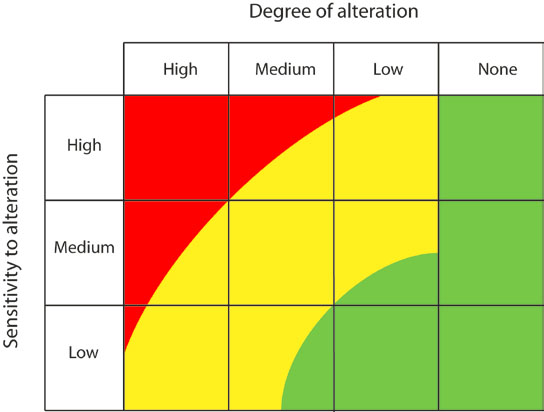
Once the potential magnitude of change for each physical indicator variable has been summarised in Table 2, the results are used to predict the changes expected in each biological indicator variable. This may be best accomplished by evaluating the impact of changes in each physical indicator variable on the biological indicator variable. Predicted changes are based on knowledge of the sensitivity of biological indicator variables to the alteration which may differ among indicators and sites (Figure 4). This process includes identifying areas where mitigation in the magnitude of alteration in any one, or combination of, indicator variable(s) can lessen the potential change in a biological indicator variable. Mitigation measures may include changes to the development’s construction footprint, its potential to cause fragmentation, and the operating plan.
Table 2: Summarising potential biophysical consequences of an alteration (see Appendix 2 for a complete table with all the indicators)
- Key ecosystem component
- Characteristic
- Indicator(s)
- Degree of alteration at the current state: Low
footnote 1 - Degree of alteration at the current state: Medium
footnote 1 - Degree of alteration at the current state: High
footnote 1 - Degree of alteration at the predicted state: Low
footnote 2 - Degree of alteration at the predicted state: Medium
footnote 2 - Degree of alteration at the predicted state: High
footnote 2 - Expected state with new alteration
- Biophysical consequences
- Confidence in the prognosis: Low
- Confidence in the prognosis: Medium
- Confidence in the prognosis: High
- Degree of alteration at the current state: Low
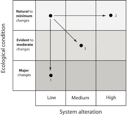
After predicting the changes to biological indicators (Table 2), this information can be evaluated to predict the overall expected change to the ecological condition of the system (conceptually illustrated in Figure 1). The response of an ecosystem to a given level of alteration will vary depending on the sensitivity of the system (Figure 4). For example, in some cases, a relatively low level of system alteration may result in a large change in ecological condition (e.g. a low level of flow alteration results in the loss of critical spawning habitat for a VEC). This situation is illustrated as trajectory 1 in Figure 5; the ecological condition of a natural ecosystem experiences major changes despite a relatively low level of alteration. Alternatively, if an ecosystem is highly resilient, a relatively large system alteration may have a minimal impact on ecological condition (illustrated as trajectory 2 in Figure 5). Between these extreme situations the change in ecological condition may directly respond to system alteration; for example, a medium level of system alteration results in a moderate change to ecological condition (illustrated by trajectory 3 in Figure 5). Translating the predicted changes in biological indicators that may result from the proposed alteration into a predicted shift in ecological condition will require interpretation and consultation on a site specific basis. Cumulative or compensatory effects of other alterations to the system need to be considered.
4.5 Post alteration monitoring
Monitoring is required to detect changes in the ecological condition of the river and valued ecosystem components resulting from alteration and to determine the effectiveness of mitigation measures. Post-alteration monitoring will also provide a better knowledge base and improve our confidence in predicting ecological impacts of future developments, including their design and operation.
For every in-stream development, a monitoring plan should be used to evaluate the effectiveness of mitigation strategies and the facility’s ultimate effect on ecosystem condition and any valued ecosystem components, such as fish populations. It is recommended that all monitoring plans include:
- The purpose of the monitoring;
- The scope of monitoring based on objectives of the operating plan, in the case of a dam, and the associated zone of influence;
- The key ecosystem components and indicators being monitored. Indicators selected for monitoring may focus on those expected to have a high or medium degree of alteration;
- The methods and procedures to be used and the level of accuracy required;
- The sampling frequency for each indicator variable (e.g. hourly, daily, weekly, monthly) and the expected duration (in years) of the monitoring program. The sampling frequency and duration are intended to capture effects of alterations that are immediate (i.e. behavioural responses to flow changes), moderate (i.e. changes to biota, communities), and long term (i.e. geomorphological evolution of the river). Rates of change in key ecosystem components are likely to be greatest immediately after alterations occur, then decline with time. Therefore, use of a monitoring schedule that gradually increases the time between sampling periods (sampling in years 1, 2, 3, 5, 7 and 10 for example) is recommended for all indicators except those specifically requiring continuous annual sampling (i.e. flow and temperature).The frequency and duration of monitoring may also be adjusted based on the perceived potential change to the aquatic ecosystem’s ecological condition. This could include the extension of monitoring activities if unanticipated effects are discovered; and
- Reporting and data availability requirements, including detailed descriptions of the study and sampling areas, the methodologies employed, the data collected, and the results and interpretation of those results.
The sampling design and indicators discussed in Section 5.3 to characterise the current ecosystem state may be used in the planning of these monitoring programs. This would ensure consistent and comparable data to best detect change in indicator variables with greatest confidence. Additional indicators and/or greater sampling intensity may be required based on site specific concerns.
Monitoring plans need to consider confounding factors that influence aquatic ecosystems, but are unrelated to the alteration (e.g. stress from recreational fishing), can be identified and taken into account during analysis of management efforts. It is also important to consider whether observed changes in indicator values during operation are related to natural variability in the system or reflect real effects from development or the effectiveness of mitigation strategies. In order to do this, the monitoring of one or more ‘control’ sites as a reference is recommended.
Appendix 1: Underlying ecological concepts
In-stream developments alter natural processes in ways that will change aquatic ecosystems. This assessment framework takes a holistic approach to assess alterations to riverine ecosystems using the following ecological concepts:
1 Ecosystem condition and integrity
Ecosystems are complex organizations of biotic communities, their physical and chemical environment, and the processes and interactions that maintain them. Sustaining aquatic ecosystems requires that both the structure and function of these ecosystems be protected. Ecological condition is a broad, holistic concept for describing the state of ecosystems as characterized by their structure and function. Ecosystem integrity refers to a condition or environmental state when the structure (e.g. species composition) and function (e.g. nutrient cycling) of an ecosystem are maintained over time (Karr 1999). Ecosystems with high integrity are composed of interconnected elements of physical habitat, and the processes that create and maintain them, ensuring these areas are capable of sustaining the full range of biota adapted for that region (Covich et al. 2005). Key characteristics of these ecosystems include intact structural elements such as species composition, native biodiversity, and variety in habitat types, and functional processes such as energy flow, material transport and hydrological processes (Karr 1991; Maddock 1999; Bain et al. 2000).
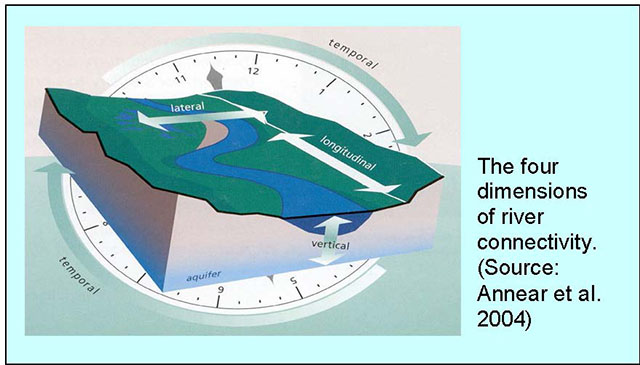
2 Connectivity
Connectivity in river systems refers to the flow, exchange and pathways that move organisms, energy and matter through the system. River system connectivity is considered to be four dimensional: the longitudinal dimension refers to the upstream- downstream connection within the river, the lateral dimension refers to the river’s connection to the riparian and floodplain areas, the vertical dimension refers to the connection between surface and groundwater, the hyporheic zone of the river bed, and finally the temporal dimension refers to the change over time in the relative importance of different river processes (Ward 1989).
Depending on their design, structures such as dams can alter connectivity and change the river’s physical and biological processes. Modifications to physical processes include changes to flow, sediment and thermal regimes and water quality. For example, altering a river’s connectivity may accelerate the erosion and sedimentation of river beds and banks, change downstream water temperatures, and enhance or impair riparian vegetation (Collier et al. 1996). These physical and chemical alterations, in turn, affect biological communities within the rivers (e.g. invertebrate and fish guilds).
Structures such as dams can also fragment and isolate biological communities by reducing or eliminating connectivity between reaches and rivers (Auer 1996; Bevelhimer 2002). For example, migratory species such as salmon may lose access to upstream habitat (Welcomme et al. 1989; Poddubny and Galat 1995; MacGregor et al. 2009) unless measures such as effective fishways are present to facilitate their upstream movement. Similarly, populations of some aquatic organisms may become isolated in areas that don’t have suitable habitat for all life stages of the species (Beamesderfer 1998). In addition, downstream connectivity can be affected by turbine mortality, which could affect populations of catadromous species, like American Eel (Verrault and Dumont 2003; MacGregor et al. 2009).
3 Natural variability
Ecosystems are dynamic and function within a range of natural variation; a state referred to as dynamic stability or dynamic equilibrium. (Resh et al. 1988) Native biota and riverine communities have evolved with, and adapted to, this dynamic stability (Poff et al. 1997; Stanford et al. 1996) which gives ecosystems the resilience to adjust to changes within this natural range. This resilience is maintained when ecosystem structure and function are intact, helping to ensure the long-term sustainability of a system. Hence, the integrity of flowing water systems depends largely on this natural dynamic character (Poff et al. 1997). Managing an ecosystem within its range of natural variability is a way to maintain diverse, resilient, productive and healthy ecosystems (Swanson et al. 1993).
4 Resilience
Resilience is a measure of the ability of species and ecosystems to persist in the presence of perturbations to the system resulting from natural (e.g. climate, fire, species invasions) or anthropogenic causes (Holling 1973). Resilient systems are able to maintain their ecological integrity when perturbed or altered even if characteristics of the systems (e.g. species abundance) aren’t constant over time. Rivers have naturally variable physical conditions and riverine ecosystems must be resilient to this variability. It is expected that these ecosystems will also be resilient to physical alterations, depending on the type and magnitude of alteration. Monitoring ecosystem integrity should therefore focus on measurements of structure and function of the ecosystem rather than the stability of selected indicators (e.g. population size).
Appendix 2: Indicator assessment table
| Characteristic | Indicator(s) | Degree of alteration at the current state | Degree of alteration at the predicted state | Expected state with new alteration | Biophysical consequences | Confidence in the prognosis: Low, Medium, High |
|---|---|---|---|---|---|---|
| Baseflow | Monthly median baseflow magnitude. | |||||
| Subsistence flow | Monthly 95% exceedance flow magnitude of total streamflow | |||||
| % wetted perimeter | ||||||
| High flow pulses < bankfull | Monthly median frequency and duration (days) of flow events less than the bankfull flow magnitude | |||||
| Channel forming flow | Magnitude, duration and timing of flows with a recurrence interval of 1.5 years | |||||
| Riparian flow | Magnitude, duration and timing of flows with recurrence intervals of 2, 10, and 20 years | |||||
| Rate of change of flow | Monthly median rate-of-change of flow for rising and falling limbs of flow events |
| Characteristic | Indicator(s) | Degree of alteration at the current state | Degree of alteration at the predicted state | Expected state with new alteration | Biophysical consequences | Confidence in the prognosis: Low, Medium, High |
|---|---|---|---|---|---|---|
| Sediment transport – Suspended | Mean annual suspended sediment yield | |||||
| Sediment transport – Bedload | Annual bankfull flow duration | |||||
| Annual excess shear power | ||||||
| Channel form and habitat | Sinuosity index | |||||
| Mean width-depth ratio | ||||||
| Bed composition |
| Characteristic | Indicator(s) | Degree of alteration at the current state | Degree of alteration at the predicted state | Expected state with new alteration | Biophysical consequences | Confidence in the prognosis: Low, Medium, High |
|---|---|---|---|---|---|---|
| Dissolved gases | Dissolved oxygen concentration | |||||
| Total dissolved gases | ||||||
| pH | pH | |||||
| Alkalinity | Alkalinity | |||||
| Conductance | Specific conductance | |||||
| Dissolved solids | Total dissolved solids | |||||
| Suspended solids | Total suspended solids | |||||
| Turbidity/light transmission | Nephelometric Turbidity (NTUs) | |||||
| Secchi disk depth | ||||||
| Nutrients | Total Phosphorus | |||||
| Total Kjeldahl Nitrogen | ||||||
| Nitrate/Nitrite | ||||||
| Total Ammonia | ||||||
| Organic matter | Dissolved Organic Carbon | |||||
| Primary productivity | Chlorophyll-a |
| Characteristic | Indicator(s) | Degree of alteration at the current state | Degree of alteration at the predicted state Low, Medium,High | Expected state with new alteration | Biophysical consequences | Confidence in the prognosis: Low, Medium, High |
|---|---|---|---|---|---|---|
| Guild | Summer thermal class (June, July and August) | |||||
| Timing | Mean annual date of maxima and minima | |||||
| Monthly modal hour of daily maxima and minima | ||||||
| Magnitude | Mean annual maxima and minima | |||||
| Monthly means of daily maxima and minima | ||||||
| Variability | Mean annual temperature range | |||||
| Monthly means of daily temperature range | ||||||
| Rate of change | Monthly means of daily maximum hourly rates of change (positive and negative) | |||||
| Duration | Species specific temperature duration ±2 °C of preferred temperatures and ≥ lethal |
| Characteristic | Indicator(s) | Degree of alteration at the current state | Degree of alteration at the predicted state | Expected state with new alteration | Biophysical consequences | Confidence in the prognosis: Low, Medium, High | ||||||
|---|---|---|---|---|---|---|---|---|---|---|---|---|
| Fish | Fish presence and absence | |||||||||||
| Fish community composition | ||||||||||||
| Index of abundance for VECs | ||||||||||||
| Size structure | ||||||||||||
| Young of year (YOY) index of abundance | ||||||||||||
| YOY growth | ||||||||||||
| Methyl mercury in fish tissue | ||||||||||||
| Benthos | Composition and abundance of dominate invertebrates | |||||||||||
| Percentage Anisoptera Plecoptera Trichoptera Ephemeroptera | ||||||||||||
| Basal resources | Biomass of coarse particulate organic matter | |||||||||||
| Periphyton: Biomass of attached algae | ||||||||||||
| Coverage of aquatic macrophytes | ||||||||||||
Chapter 2: Hydrologic regime
List of acronyms
- AABI
- Absolute annual baseflow index
- AFI
- Annual flow index
- AMS
- Annual maximum series
- APR
- Approval and Permitting Requirements
- FDC
- Flow duration curve
- FDCI
- Flow duration curve index
- FFA
- Flood frequency analysis
- FFC
- Flood frequency curve
- HBV
- Hydrologiska Byråns Vattenbalansavdelning
- IQR
- Interquartile range
- MBI
- Monthly baseflow index
- MMB
- Median monthly baseflow
- OLWR
- Ontario Low Water Response
- PDS
- Partial duration series
- PEI
- Percent exceedance index
- SAAS
- Streamflow Analysis and Assessment Software
- VEC
- Valued ecosystem component
- WPF
- Waterpower facility
- WSC
- Water Survey of Canada
1.0 Introduction
The natural hydrologic regime of rivers and lakes is the long-term unaltered pattern of flow and level magnitude, duration, seasonality (timing), frequency, and rate of change. This pattern is a strong determinant of the structure, function, and composition of aquatic ecosystems (Poff et al. 1997; Baron et al. 2002).
This chapter focuses on variables of a flow regime strongly associated with ecological condition and, therefore, most suited to serve as indicators of hydrologic alteration. Methods to quantify indicators and to assess the degree of alteration in a flow regime through time using the deviation from a reference condition (i.e. natural, least disturbed, or current flow regime) are discussed. This provides a common reference from which to monitor change in the flow regime through time and to help explain changes in ecological condition.
Hydrology is tightly linked to other riverine processes. Therefore the strong association between hydrologic indicators and ecological condition is often traced to a specific hydrologic/hydraulic function important for processes related to other key ecosystem components. For instance, the flow regime is tightly coupled with erosion and transport processes related to the sediment regime. As such, hydrologic indictors related to these important functions are included here while specific fluvial geomorphology indicators are included in the sediment regime chapter.
2.0 Rationale
The dynamic variability of a river’s hydrologic regime organises and defines river ecosystems and their biodiversity, production, and sustainability (Poff et al. 1997). A range of flows is necessary to scour and revitalise gravel beds, to import wood and organic matter from the floodplain, and to provide access to productive riparian wetlands (Poff et al. 1997). Native biota and riverine communities have evolved with, and adapted to, the flow regime of a river system, including the seasonal and inter-annual variability that is an ecologically important part of this natural cycle (Poff et al. 1997; Stanford et al. 1996).
Flow alteration changes the pattern of natural variation and disturbance on a river system. It results in the conversion of riverine (lotic) ecosystems to lake-like (lentic) ecosystems upstream of structures such as dams and the imposition of a flow regime downstream that can be significantly different from the natural flow. Altered flow regimes, particularly those associated with the establishment of reservoirs located upstream of dams can dramatically change river system characteristics most responsible for influencing freshwater ecosystems (Baron et al. 2002). In-stream developments change the distribution of flow magnitude, duration, frequency, seasonality, and rates of flow increase and recession. The degree and type of flow modification depends upon the purpose of the development. For waterpower facilities, these modifications can range from subtle changes downstream of run-of-river facilities to large diurnal fluctuations downstream of peaking facilities, with effects on the riverine ecosystem varying accordingly. Such modifications are now recognized as one of the primary causes of aquatic ecosystem alteration related to waterpower development (Moog 1993; Lind et al. 2007).
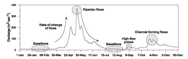
Each aquatic ecosystem requires a certain amount of water to maintain its ecological integrity. In very broad terms, these environmental water requirements can be defined as the quantity and quality of water required to protect the structure, function, and species composition of that ecosystem. Satisfying these requirements, while at the same time accommodating other water uses, ensures ecologically sustainable development. Thus, whenever possible the aim of environmental water requirements is to maintain or restore a degree of hydrologic variability to altered systems that incorporates important components observed in natural flow and level regimes and that serve important ecological functions for a healthy natural environment. A more natural degree of hydrologic variability (i.e. the reference condition) is conducive to sustaining the ecological integrity of aquatic ecosystems (Poff et al. 1997; Arthington et al. 2006), or preventing degradation in ecological condition. Components of flow regimes considered important for maintaining the ecological condition of riverine ecosystems are described in Table 1, while important characteristics commonly used to define their pattern are described in Table 2. When characteristics of these flow components are integrated into altered flow regimes to achieve aquatic ecosystem objectives, they are often referred to as environmental flows. The implementation of these environmental flows is thus based on the premise that: 1) the flow components can be identified, isolated, and characterized using a historic or reference flow regime; 2) biophysical consequences of altering these flow components are known; and 3) biophysical consequences can be used to predict potential change to river condition (Brown and King 2000).
3.0 Indicator summary
Hydrologic components and associated indicators described in this chapter to evaluate hydrologic alteration (Figure 1 and Table 3) mirror the environmental flow components and associated characteristics shown in Tables 1 and 2. It should be emphasized that small deviations in each indicator from the reference condition may not necessarily equate to lower degradation in ecological condition. Alteration may still exist that is not explained by the given indicators and there may be cumulative and synergistic effects that may still pose a risk to ecological condition. A more thorough assessment of the hydrologic alteration can be conducted during post-alteration monitoring when continuous streamflow records would be available to assess the entire flow regime. In these instances, indicators identified in Table 3 can be supplemented with more comprehensive indices of alteration that examine the flow regime in its entirety and provide a better assessment of the alteration from the reference condition or through time (see Section 7).
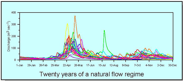
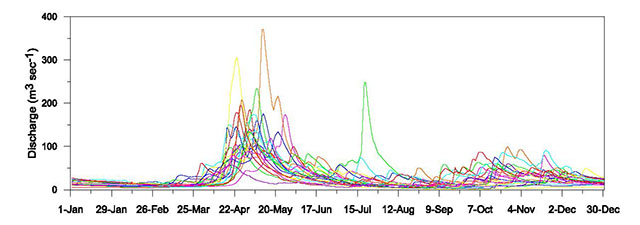
4.0 Establishing a reference
The natural flow regime is the unaltered river’s pattern of flow quantity, timing, and variability as observed over any time scale using many years of data (Poff et al. 1997) (Figure 2). The natural flow paradigm has been developed on the premise that the ecological integrity of flowing water systems depends on their natural dynamic character and that deviations from a natural flow regime may act as indicators of ecological impairment (Poff et al. 1997). Estimated deviations from a natural flow regime resulting from an in-stream development can thus be used to evaluate the extent of alteration to a system and the potential effect on ecological condition. Deviations from a natural flow regime can also form the basis for mitigation measures (e.g. maintaining a baseflow) intended to minimize impairment of ecological condition.
| Flow component | Description | Ecological function |
|---|---|---|
| Overbank flows | Infrequent, high flow events that exceed the normal channel. | These flows shape and redistribute physical habitats, purge invasive species, provide lateral connectivity between the channel and the active floodplain, provide life-cycle cues for various species, and facilitate exchange of nutrients, sediments and woody debris. |
| High flow pulses | Short-duration, in-channel, high flow events. | These flows maintain physical habitat by flushing silt and fines and preventing the encroachment of riparian vegetation into the channel, providing lateral connectivity to oxbows and providing life-cycle cues for various species. |
| Low flows | Normal flow conditions between high flow events sustained through the release of surface and groundwater storage. | These flows maintain water tables for riparian vegetation (lateral connectivity), provide longitudinal connectivity, and provide a range of suitable habitat conditions that maintain the diversity of the natural biological community. |
| Subsistence flows | Infrequent, naturally occurring low flow events of long duration (occurring over seasons). | These flows maintain sufficient water quality and provide sufficient habitat and connectivity to prevent direct mortality of aquatic species and ensure survival of organism populations capable of recolonising the river system once normal baseflow returns. |
| Flow characteristic | Description |
|---|---|
| Magnitude | The amount of water moving past a fixed location per unit time. |
| Frequency (of occurrence) | How often a flow above a given magnitude occurs over some specified time interval. |
| Duration | The period of time associated with a specified flow condition. |
| Timing | The predictability of flows of defined magnitude; the regularity at which they occur. |
| Rate of change (ramping rate) | How quickly flow changes from one magnitude to another. |
| Characteristics | Indicator(s) |
|---|---|
| Baseflow | Monthly median baseflow magnitude (m3sec-1). |
| Subsistence flow | Monthly 95% exceedance flow magnitude of total streamflow (m3sec-1) (preliminary assessment) % wetted perimeter (field-based assessment) |
| High flow pulses (less than bankfull) | Monthly median frequency and duration (days) of flow events less than the bankfull flow magnitude |
| Channel forming flow | Magnitude (m3sec-1), duration (days) and timing (month) of flows with a recurrence interval of 1.5 years |
| Riparian flow | Magnitude (m3sec-1), duration (days)and timing (month) of flows with recurrence intervals of 2, 10, and 20 years |
| Rate of change of flow | Monthly median rate-of-change of flow (m3sec-1hr-1) for rising and falling limbs of flow events. |
The first step to establish a reference condition is to obtain/model the natural or least disturbed flow pattern at the site of the proposed alteration in the form of continuous daily streamflow time series (Appendix 1, Section 1). The reference condition time series should be simulated for the location on the river immediately downstream of a development (planned or existing) where all diverted and non-diverted water converges (i.e. from the tailrace, spill channels, and any bypassed natural channel reaches of an in-stream diversion). It is at this point where the hydrologic alteration caused by the development is fully integrated. The assessment criteria derived from this reference time series would also apply to the bypassed natural channel reach, unless the differences in drainage basin areas from the top to the bottom of the diversion is significant enough to suggest that the mean annual flow would be different at those two locations on the river. In that case, a second reference condition time series would be necessary for the location on the river where the diversion will begin.
From the simulated reference condition time series, hydrological assessment criteria can be quantified. Ideally, the resolution of the time series should be sufficient to capture the full pattern of flow at a site. Smaller rivers that respond more quickly to rainfall events would require higher resolution (hourly or less) to capture changes in flow. The pattern of flow in larger, less responsive rivers where differences in hourly instantaneous flow during a day are minimal, might be adequately represented with daily average flow (see Appendix 1, Section 3.2). Although it is recognised that at least 20 years of streamflow data is preferable to adequately characterise the natural pattern of flow for the reference condition (see Appendix 1, Section 1.1), the length of altered flow time series to be used for assessments will depend entirely on the specific questions being asked and the assessment period of interest.
5.0 Information requirements
The information requirements and associated data needs identified in Table 4 support the assessment of hydrologic alteration.
If the reference condition for a site with a natural flow regime (i.e. a greenfield site) is developed using proration, spatial interpolation or a hydrologic model (see explanations in Appendix 1), streamflow monitoring at the site of the proposed alteration can be used to increase the accuracy of the simulated flow regime. Streamflow data can be correlated with historical flow records to improve proration and spatial interpolation methods or for validating/optimising a hydrologic model (see Appendix 1, Section 1.1). The monitoring period should be a minimum of 12 months to capture the annual distribution of flows but most sites likely require a minimum of 24 months because of interannual variability. The longer the time series, the more variability can be captured in the streamflow, increasing certainty in the results. The improved simulated flow regime can then be used to recalculate the assessment criteria for each indicator. Hydrometric field techniques to complete this monitoring are discussed in Appendix 1, Section 1.3.
| Information requirement | Data need |
|---|---|
| Assessment criteria values for the reference condition | Historical streamflow data or climate data and basin characteristics depending on the method used to simulate a natural reference condition (daily streamflow simulation). Field-based measurements of streamflow to improve the accuracy of the streamflow simulation. |
| Indicator values for the current condition (if already altered) | Hourly streamflow data from an existing facility or stream gauge(s). |
| Indicator values for the proposed post-alteration condition. | Information on the proposed design and operation of the facility as it pertains to the passage of water. |
For new alterations, the hydrologic indicators would be estimated from knowledge of the proposed design and operation of the facility. The possible degree of alteration would be evaluated by comparing these estimates to the assessment criteria values derived from the reference condition. For rivers with existing in-stream developments, a discharge time series would ideally be available from one of the structures that could be used to derive hydrologic indicators for the current (altered) condition. This would include time series for waters passing through any waterpower facility, a spillway, and bypassed natural channel reach. The latter would be used to establish the current hydrologic condition of the reach while the integration of all three time series could be used to establish the current altered condition downstream of the structure. Otherwise, hydrometric stations can be used to establish the streamflow time series in the bypassed reach and downstream of the structure.
The hydrologic alteration in bypassed natural channel reaches may be significant, so assessing the deviation from the reference condition is important to identify ecological functions that may be affected in these reaches. Subsistence flow indicators will be particularly important in these reaches. Specific information requirements for indicators are discussed in the respective sections below.
6.0 Streamflow characteristics, indicators, and assessment criteria
Methods to calculate hydrologic indicators and assessment criteria for flow regimes as part of the framework described in Chapter 1 are provided below. Given hydrological data are typically neither independent nor normally distributed and often contain extreme values, non-parametric statistics have been selected to characterise the central tendency (indicators) and variability (assessment criteria) in the data. In Figure 3, measures of dispersion around the median are shown as percent exceedances – a common convention used by hydrologists when analysing flow duration curves (FDCs). The percent exceedance is obtained by subtracting the percentile scale value from 100 percent. For example, a discharge at the 75 percent exceedance is the same as a discharge at the 25th percentile (100-25=75). In keeping with this convention, percent exceedance will be used to describe values associated with a flow duration curve while percentiles will used to describe all other data. Figure 3 also shows the associated levels of alteration with increasing distance from the median. The values demarcating the boundaries between the alteration levels have been rounded to simplify assessment criteria calculations.
In some cases, indicators and assessment criteria will be calculated using preliminary assessments, primarily desk-top methods, and refined, or in some cases replaced, with field-based assessments when such data can be collected. Most indicator metrics and assessment criteria can be obtained using the Streamflow Analysis and Assessment Software (SAAS) to analyse either an altered or natural reference streamflow time series. A table is provided at the end of Appendix 1 to organise all values for indicators and assessment criteria and to assist in the overall evaluation of hydrologic alteration. These can then be summarised in the Table included in Chapter 1 Appendix 1.
6.1 Baseflow
6.1.1 Description and rationale
Streamflow is maintained by a combination of surface runoff and baseflow components. Baseflow is defined as the streamflow portion contributed by persistent, slowly varying sources (i.e. groundwater, lakes, wetlands) between precipitation events (Dingman 1994). Temporally variable baseflow conditions in rivers are important for maintaining ecosystem function. Baseflow provides a relatively stable supply of high quality water, relatively constant in temperature, which is important to stream biota that have become adapted to the timing and quantity of these inputs (Bunn and Arthington 2002; Neff et al. 2005). The role of baseflow in maintaining streamflow between episodic flow events (e.g. spring melt and rain events) has resulted in it being considered an important ‘ecological reserve’ flow (Smakhtin 2001).
The magnitude of baseflow relative to total streamflow is often used to characterise the relative importance of contributions from these sources. These contributions define a river’s baseflow regime, and are influenced by a number of natural factors including the rate, frequency, and amount of groundwater recharge and discharge, soil characteristics, topography, hydrogeology and hydraulic characteristics of aquifers, evapotranspiration rates, area of surface water storage, and climatic variability (Smakhtin 2001). Throughout the better part of the drier periods, discharge is comprised entirely of baseflow. A comprehensive review of baseflow hydrology has been completed by Smakhtin (2001).
Numerous studies have associated the use of the term baseflow with a low flow, environmental flow, ecological flow or instream flow target (Tennant 1976; Wallace and Cox 2002; Hayes and Nelms 2001; Petts et al. 1997; Ries 1997; Smakhtin 2001; Environmental Protection Agency 2003; Harman and Stewardson 2005). An array of statistical methods have also been used to estimate baseflow magnitudes for hydrologically-based environmental flows. These are popular because of their relative ease of calculation and include examples such as a percentage of the mean annual flow (MAF) (e.g. Tennant 1976; Tessman 1980) and percent exceedance from a FDC (Annear et al. 2004). The use of simplistic prescriptive environmental flow targets based on percentages of annual flows have been criticized as having no documented empirical basis and represent a “grave risk to the future integrity and biodiversity of the worlds riverine ecosystems” (Arthington et al. 2006). Employing baseflow separation methods to directly quantify the baseflow contribution to the total streamflow hydrograph provides a more intuitive hydrology-based method of charactersising this flow component and calculating associated indicators and assessment criteria (Brown and King 2000). This moves away from methods that calculate baseflow as a ‘minimum flow’ target with magnitudes resembling extreme events, a practice Smakhtin (2007) refers to as “unsound”. The method to calculate baseflow indicators described here is premised on the assertion that quantifying actual baseflow values using observed or modelled streamflow provides the best indicator for this environmental flow. Baseflow separation is discussed in Appendix 1, Section 1.2.
6.1.2 Indicators
Baseflow indicators include the monthly median baseflow (m3sec-1).
This indicator is calculated using the median of all daily or hourly baseflow values for each month for the period of record (e.g. the median baseflow of all Januaries in the period of record, etc.). The median baseflow is the most appropriate measure because it is less influenced by extreme events (i.e. high and low baseflows) and therefore, better represents typical streamflow conditions. Summarising the data on a monthly time-scale is sufficient to characterise the annual variability in baseflow. The ecological importance of intra-annual variation in baseflow would be dampened considerably if baseflow values were aggregated by seasons and its importance eliminated entirely if only an annual value was estimated.
6.1.3 Information requirements
Calculation of baseflow indicators for the reference condition requires a baseflow time series extracted from a natural flow simulation at the site of the flow alteration. Baseflow separation is discussed in Appendix 1, Section 1.2. If the initial reference condition time series was improved using streamflow monitoring from the site, the baseflow separation and calculation of assessment criteria indicator values should be repeated.
6.1.4 Assessment criteria
Assessment criteria for baseflow indicators include the monthly baseflow values associated with the 13th, 38th, 62nd, and 87th percent exceedances, calculated using the reference condition baseflow time series (Figure 3).
6.1.5 Evaluating alteration
The degree of alteration in individual indicators can be evaluated as follows:
Low alteration: A monthly median baseflow indicator that lies between the 38th and the 62nd percent exceedance baseflow for the reference condition.
Medium alteration: A monthly median baseflow indicator that lies between the 13th and 38th or 62nd and 87th percent exceedance baseflow for the reference condition.
High alteration: A monthly median baseflow indicator less than the 13th or greater than the 87th percent exceedance baseflow for the reference condition.
Total baseflow alteration should be evaluated by assessing the suite of monthly indicators together. For instance, low alteration would be associated with monthly indicator values distributed equally above and below the median monthly baseflow in ‘average’ flow years, biased toward the 62nd percent exceedance in ‘dryer’ years and toward the 38th percent exceedance in ‘wetter’ years. Thus, monthly indicator values that lie between the 38th and the 62nd percent exceedance baseflow of the reference condition but constantly in the lower range (i.e. close to the 62nd percent exceedance) might warrant an adjustment from low to medium alteration. Transitions from one monthly baseflow magnitude to the next should avoid rapid changes that may harm biota (e.g. stranding of fish).
6.1.6 Methods
To determine the flow magnitudes associated with the baseflow indicators and assessment criteria, the 13th, 38th, 62nd, and 87th percent exceedance values are calculated for each month of the period of record. That is, for twenty years of a simulated flow regime a baseflow separation is performed and used to calculate the daily baseflow magnitudes that are then aggregated into their respective months (e.g. all daily values for each January for 20 years = 620 values) and a single period-of-record baseflow duration curve produced for each of the 12 months of the year. Values for indicators and assessment criteria are obtained from the baseflow duration curve for each month (Figure 4).
6.1.7 Adjusting the timing for transitioning between monthly baseflow
The timing of seasonal hydrologic events varies and seldom aligns with calendar months. This is most noticeable on the rising and falling limb of springmelt and autumn flows. Thus, the dates for transitioning between environmental baseflows of different magnitude should be flexible enough to adjust to the timing of the rising and falling limbs of these events and adjusted accordingly.
6.2 Subsistence flow
6.2.1 Description and rationale
The baseflow indicators and assessment criteria use the full baseflow time series to characterise average baseflow conditions (i.e. from the smallest to the largest magnitudes). However, all flow regimes contain infrequent, naturally occurring low flow events of long duration where baseflow is at its lowest magnitude. These extreme low magnitude baseflows, or subsistence flows, require specific consideration because of their importance for maintaining sufficient water quality, habitat, and connectivity in the river until normal baseflow conditions return. Subsistence flow indicators and assessment criteria are important to characterise as they provide an indication of flow conditions that might be expected under extreme drier conditions but which maintain important ecological functions for the survival of aquatic species and the ecological condition of river systems.
When assessing hydrologic alteration for bypassed natural channel reaches resulting from instream diversions, it is important to validate, through field observations, whether subsistence flow indicators would indeed satisfy the important ecological functions and water requirements of valued ecosystem components (VECs) identified for the reach. Subsistence flow indicator values should be adjusted upwards if necessary for defined periods to meet specific VEC water requirements (e.g. migration and spawning of fish) before estimating the potential hydrologic alteration.
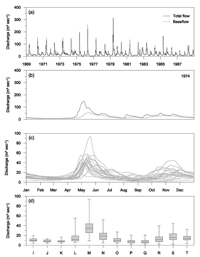
6.2.2 Indicators
6.2.2.1 Preliminary assessment
The subsistence flow indicator is the stream flow magnitude (m3sec-1) equal to the monthly 95 percent exceedance flow using total streamflow.
The 95 percent exceedance flow is a commonly used indicator of extreme low flow conditions (Brilly et al. 1997; Smakhtin 2001; and Tharme 2003) and considered to be the minimum flow magnitude required to protect a river (Petts et al. 1997). The calculation of monthly subsistence flow indicators is important since a flow magnitude associated with the 95 percent exceedance flow in August may not provide the same ecological function under winter conditions.
6.2.2.2 Field-based assessment
The subsistence flow indicator is the stream flow magnitude (m3sec-1) that covers 50% of the wetted perimeter for rivers < 15m wide and 70% of the wetted perimeter for larger rivers.
Observations show that discharges calculated using these wetted perimeter methods to be similar to the 90-95 percent exceedance flow extracted from period-of-record flow duration curves of total flow (Annear et al. 2004). Similarly, period-of-record exceedance values for the streamflow magnitudes associated with the field-based assessment indicators should also be recorded.
6.2.3 Information requirements
6.2.3.1 Preliminary assessment
Calculation of the subsistence flow indicator requires a natural flow time series (reference condition) at the site of the flow alteration. Recommended methods for establishing the reference condition are provided in Appendix 1, Section 1.1. Baseflow separation is discussed in Appendix 1, Section 1.2.
6.2.3.2 Field-based assessment
Required field measurements include surveying cross sections at riffles (thought to be the most critical habitat) in the bypassed reach that extend from the bankfull stage on one side to the bankfull stage on the other side. The distance along the stream bottom from the wetted edge on one bank to the wetted edge on the other bank should be recorded (measured or modelled) at a range of discharges and the wetted perimeter (y-axis) vs discharge (x-axis) relationship graphed. If modelled, field measurements of wetted perimeter at a range of discharges should be used for validation.
6.2.4 Assessment criteria
Unlike assessment criteria for other indictors, those for the subsistence flow are based on extreme conditions and not the deviation from the natural baseflow.
Assessment criteria for the subsistence flow indicator includes the baseflow values associated with the 95 and 99 percent exceedance using monthly period-of-record FDCs from the reference condition streamflow time series.
6.2.5 Evaluating alteration
Alteration in individual indicators is evaluated as follows:
Low alteration: A subsistence flow indicator (m3sec-1) > the 95 percent exceedance flow of the monthly FDC for the period-of-record from the reference condition streamflow time series or a streamflow magnitude that covers ≥ 50% of the wetted perimeter for rivers < 15m wide or ≥ 70% of the wetted perimeter for larger rivers.
Medium alteration: A subsistence flow indicator (m3sec-1) > 99 percent exceedance of the monthly FDC for the period-of-record from the reference condition streamflow time series.
High alteration: A subsistence flow indicator (m3sec-1) < 99 percent exceedance of the period-of-record monthly FDC from the reference condition streamflow time series or a streamflow magnitude that covers < 50% of the wetted perimeter for rivers < 15m wide or < 70% of the wetted perimeter for larger rivers.
6.3 High flow pulses (less than bankfull)
6.3.1 Description and rationale
High flow pulses are distinct flow events identifiable in the streamflow time series that are perched upon baseflow but are less than the bankfull flow magnitude. These smaller events are the result of lower intensity rain events, short winter or spring thaws, or rain events occurring during drier conditions (i.e. more available storage in the basin). High flow pulses are important for regular maintenance of physical habitat by flushing silts and fines from river beds and preventing encroachment of riparian vegetation. They can stimulate spawning of fish, flush out poor quality water, mobilize and sort gravels, and contribute to maintaining heterogeneity of physical biotopes (King et al. 2003)
6.3.2 Indicator
High flow pulse indicators include the monthly median frequency of flow events less than the bankfull flow magnitude (see Section 6.3) and the monthly median duration (median, measured in days) for the period of record.
The high flow pulse indicators are calculated using flow events for each month for the period of record. For example, the frequency of events for each January is tabulated for the period of record (e.g one number for each year being analysed) and the median frequency for January calculated. The median duration is calculated for all of January flow events for the period of record at once (i.e. without summarising annually first).
6.3.3 Assessment criteria
Assessment criteria for the high flow pulse indicators include the monthly frequency and duration magnitudes (days) associated with the 13th, 38th, 62nd, and 87th percentiles calculated using the reference condition streamflow time series.
6.3.4 Evaluating alteration
The degree of alteration in individual indicators can be evaluated as follows:
Low alteration: Monthly median high flow pulse frequency and duration indicators that lie between the 38th and the 62nd percentiles, respectively, for the reference condition.
Medium alteration: Monthly median high flow pulse frequency and duration indicators that lie between the 13th and 38th or 62nd and 87th percentiles, respectively, for the reference condition
High alteration: Monthly median high flow pulse frequency and duration indicators that are less than the 13th or greater than the 87th percentile, respectively, for the reference condition.
6.3.5 Methods
High flow pulses are distinct flow events that can be identified between the bankfull flow magnitude and baseflow using quantitative thresholds (i.e. peak to baseflow ratio). Once identified, monthly counts and flow event duration are used to determine the high flow pulse frequency and duration. Criteria and methods for identifying high flow pulses using quantitative thresholds have been included in the Streamflow Analysis and Assessment Software (SAAS).
6.4 Channel-forming flow
6.4.1 Description and rationale
Channel-forming flows are those that surpass the threshold of sediment erosion and movement. They produce a diverse natural channel structure that includes features such as bars, riffle-pool sequences, and varying width and depth which are all important for maintaining healthy riverine ecosystems (Bayley 1995; Stanford et al. 1996; King and Louw 1998). These include rain-induced flow events and those associated with springmelt runoff. Channel-forming flows, also referred to as channel maintenance flows, flushing flows, or dominant discharge have most commonly been associated with the bankfull flow stage (depth of flow). At this stage, water just begins to overflow onto the floodplain, corresponding to a discharge at which channel maintenance is thought to be most effective (Dunne and Leopold 1978; Rosgen 1996; Annable 1996; Simon et al. 2004). Other definitions include:
- the flow at a river cross-section that “just fills the channel to the tops of the banks” (Williams 1978);
- the discharge which maximizes sediment transport (Andrews 1980; Carling 1988);
- the discharge associated with changes in river cross-section (Wolman 1955; Riley 1972; Williams 1978);
- dominant discharge, effective discharge, or channel forming discharge, it is the flow which performs the most work, defined in terms of sediment transport (Wolman and Miller 1960); and
- habitat maintenance flows and spawning/migration freshet flows (King and Louw 1998)
In an overview of published definitions of bankfull flow, Radecki-Pawlik (2002) recommended the definition by Williams (1978).
These definitions are all based on the premise that bankfull discharge is the flow rate at which most geomorphic work is done in a river channel. Ryan et al. (2002) and Schmidt and Potyondy (2004) suggest a value of 80% of the bankfull discharge 0.8(Q1.5) as the flow threshold that begins to move significant bedload material. Thus, bankfull river stage and the subsequent estimation of bankfull river discharge are useful conservative measures in fluvial hydrological investigation for understanding the role of these higher magnitude flows in maintaining stream habitat and the ecological condition of river systems.
In a study of 47 rivers in Southern Ontario, Annable (1994) found that bankfull discharges had a recurrence interval between 1.5 and 1.7 years. The recurrence interval is an estimate of the probability of the occurrence of a bankfull flow. For instance the 1.5 year flood is one which will, on average, be equalled or exceeded once in a one and a half year period. Thus the recurrence interval only refers to the average spacing of events over a larger number of years, not that it occurs every 1.5 years. Indeed, a bankfull flow may occur twice in a year and then not for another 3 years.
Although limited to a specific region of the Province, these results are comparable to the generally accepted recurrence interval of 1.5 years for bankfull discharge (Leopold et al. 1964; Williams 1978; Dunne and Leopold 1978; Rosgen 1996) and encompass slightly higher estimates of 1.58 years (Dury et al. 1963; Dury 1973) and 1.6 years (Page 1988). Recent work summarizing historical flow and suspended sediment data for thousands of gauging stations across the U.S. has confirmed the use of the 1.5 year recurrence interval as a good measure of effective discharge (Simon et al. 2004).
6.4.2 Indicators
6.4.2.1 Preliminary assessment
Channel-forming flow indicators useful for preliminary assessments include the streamflow magnitude (m3sec-1) associated with a recurrence interval of 1.5 years (bankfull flow), the median duration (measured in days) and timing (modal month), calculated using all flow events in the time series that equal or exceed this magnitude.
6.4.2.2 Field-based assessment
Although recurrence intervals for bankfull flow events across varying geographies are very similar, field measurements at specific sites increase certainty in their estimated magnitude.
Channel-forming flow indicators include the streamflow magnitude (m3sec-1) associated with the field estimate of bankfull stage, the associated recurrence interval (years) and the median duration (measured in days) and timing (modal month), calculated using all flow events in the time series that equal or exceed this magnitude.
6.4.3 Information requirements
Methods and associated information requirements for measuring bankfull flow stage in the field and estimating the corresponding discharge are provided in Appendix 1, Section 2.2.
Where simulated flow regimes have been improved by hydrometric monitoring in the field (Appendix 1, Section 2.1), channel-forming flow indicators for the streamflow magnitude (m3sec-1) associated with the field estimate of bankfull stage should be recalculated (e.g. recurrence interval, duration, timing).
6.4.4 Assessment criteria
Assessment criteria for the channel-forming flow indicators include the streamflow magnitude (m3sec-1) associated with a recurrence interval of 1.5 years (bankfull flow), the streamflow magnitude associated with 80% of the bankfull magnitude (m3sec-1), monthly duration values (days) associated with the 13th, 38th, 62nd, and 87th percentiles, and the distance from the modal month (measured in months) for all events meeting the magnitude criteria calculated using the reference condition streamflow time series.
6.4.5 Evaluating alteration
The degree of alteration in individual indicators can be evaluated as follows:
Low alteration: Magnitude indicators equal to or greater than the bankfull flow magnitude, duration indicators that lie between the 38th and the 62nd percentiles, and timing indicators within the same month of the reference condition.
Medium alteration: Magnitude indicators within 80% of the bankfull flow magnitude, duration indicators that lie between the 13th and 38th or 62nd and 87th percentiles, and timing indicators within one month of the reference condition.
High alteration: Magnitude less than 80% of the bankfull flow magnitude, duration indicators that are less than the 13th or greater than the 87th percentile, and timing indicators greater than two months of the reference condition.
6.4.6 Methods
Streamflow magnitudes associated with these bankfull flow recurrence intervals are determined for a site by conducting a flood frequency analysis (FFA) on the observed or simulated streamflow time series. Once the magnitude of bankfull flow is known, characteristics related to the duration and timing of these events can be determined.
Although a partial duration series (PDS) is commonly preferred to estimate the magnitude of smaller events of higher frequency and from shorter records, estimates of bankfull flow recurrence intervals obtained in the studies referenced in Section 6.2.1 were derived using the annual maximum series (AMS) and therefore an AMS should be used to calculate metrics for bankfull flow indicators. For recurrence intervals greater than 10 years, there is no significant difference between the partial-duration series and the annual-maxima series (Dunne and Leopold 1978). Likewise, the Log-Pearson III (LP3) distribution should be used in the flood frequency analysis to remain consistent with the methods of Annable (1994). Although instantaneous peak discharges are preferred for flood frequency analysis over daily average discharges which tend to underestimate flow peaks, it is recognised that the latter is likely to be more commonly available, particularly if the time series was simulated. Similarity between instantaneous daily peak values and daily average streamflow increases with increasing basin size and increasing proportion of baseflow to the total streamflow hydrograph. Thus, for smaller, bedrock basins (i.e. river systems with a ‘flashier’ response), daily averaged streamflow will underestimate the highest observed streamflow and metrics for bankfull flow indicators may be underestimated.
6.5 Riparian flow
6.5.1 Description and rationale
Riparian flows are overbank events that inundate riparian areas, resulting in significant interaction between the channel and floodplain and are responsible for maintaining biological diversity and productivity of the riverine ecosystem (OMNR 1994; Rowntree and Wadeson 1998; Nilsson and Berggren 2000; Nilsson and Svedmark 2002; Tiegs et al. 2005). Outright removal, or considerable reductions in the frequency and magnitude of riparian zone flood disturbance associated with altered flow regimes have been linked to declines in riparian and floodplain species diversity which are tightly linked to overbank flow disturbance (Pollock et al. 1998; Petit et al. 2001; Johnson 2002; Lytle and Merrit 2004). Reductions in riparian flows have also been linked to reductions in instream biological integrity caused by disruptions in trophic pathways and alterations of instream habitat (Naiman and Decamps 1997). In a study of 21 dams across the U.S., Magilligan et al. (2003) determined that riparian flows, comprised of floods greater than bankfull, have been essentially eliminated by dams, disconnecting the riparian zone from the riverine influence, and threatening the long-term ecosystem stability and biodiversity, nationally. Hence, maintaining riparian flows is integral to the biological integrity of altered riverine systems.
Under natural flow conditions riparian flow events occur between 1:2 year and 1:20 year return periods (OMNR 1994), or can be determined as flows covering the equivalent of the “confinement area” (Rosgen 1994). Recommended riparian flows are those with a magnitude that lie within this range.
6.5.2 Indicator
Riparian flow indicators include the streamflow magnitude (m3sec-1) associated with a recurrence interval of 2, 10 and 20 years, the median duration (measured in days) and timing (modal month), calculated using all flow events in the time series that equal or exceed these magnitudes.
6.5.3 Assessment criteria
Assessment criteria for the riparian flow indicators include the streamflow magnitude (m3sec-1) associated with a recurrence interval of 2, 10 and 20 years, duration magnitudes (days) associated with the 13th, 38th, 62nd, and 87th percentiles, and the distance from the modal month (measured in months) derived from the reference condition streamflow time series.
6.5.4 Evaluating alteration
The degree of alteration in individual indicators can be evaluated as follows:
Low alteration: Magnitude indicator equal to or greater than the respective recurrence interval flow magnitude, duration indicators that lie between the 38th and the 62nd percentiles, and timing within the same month of the reference condition.
Medium alteration: Magnitude indicator equal to or greater than the respective recurrence interval flow magnitude, duration indicators that lie between the 13th and 38th or 62nd and 87th percentiles, and timing within the same month of the reference condition (Note: Other combinations of indicator deviation might be considered medium alteration when taking into account a site’s sensitivity to changes in each).
High alteration: Magnitude indicator less than the respective recurrence interval flow magnitude, duration indicators that are less than the 13th or greater than the 87th percentile, and timing greater than two months of the reference condition.
6.5.5 Methods
The riparian flow indicator should be calculated by flood frequency analysis using the Log- Pearson III (LP3) distribution with an annual maxima series to maintain consistency with the calculation of the bankfull flow indicators. Note that for larger flood flows (e.g. 100 year recurrence interval), the three-parameter lognormal distribution is preferred (Ontario 2002a). The 2 year recurrence interval flow indictor provides information on flows that met the minimum threshold for a riparian flow. As described in Section 6.2.6, instantaneous peak discharges are preferred over daily average discharges. Once the magnitude of the riparian flow is known, the duration, timing, and rate of change of these events can be determined using the historical streamflow time series.
6.6 Rate of change of flow
6.6.1 Description and rationale
The rate of change of flow (m3sec-1 hr-1), either increasing or decreasing, associated with the rising and falling limbs of a rain or snowmelt event on a natural hydrograph are analogous to the up-ramping and down-ramping observed in flow regimes downstream of peaking waterpower facilities. The effect on riverine systems of operational ramping rates greater than the average rate of change of flow observed on the natural hydrograph is receiving increased attention (cf. Halleraker et al. 1999; Harby et al. 1999; Smokorowski et al. 2009). Rapid fluctuations in flow associated with ramping are known to result in physical displacement of aquatic biota, behavioural changes, and significant change in habitat (Vehanen et al. 2000; Flodmark et al. 2002). Changes to the quality of habitat are also manifested in the disturbance to the fluviogeomorphological system (e.g. stream bank erosion and sedimentation).
6.6.2 Indicator
The rate of change of flow indicators include the monthly median rate of change of flow (m3sec-1hr-1) calculated from all streamflow values for both the rising (positive) and falling (negative) limbs of identified flow events whose peaks fall within the given month.
6.6.3 Assessment criteria
Assessment criteria for rate of change of flow indicators include the monthly rate of change magnitudes (m3sec-1hr-1) (positive and negative) associated with the 13th, 38th, 62nd, and 87th percentiles calculated using the rising and falling limbs of reference condition streamflow time series.
6.6.4 Evaluating alteration
Alteration in individual indicators is evaluated as follows:
Low alteration: A monthly median rate of change of flow indicator for both positive and negative rates that lies between the 38thand the 62nd percentile rate of change of flow for the reference condition
Medium alteration: A monthly median rate of change of flow indicator for both positive and negative rates that lies between the 13thand 38thor 62nd and 87thpercentile rate of change of flow for the reference condition.
High alteration: A monthly median rate of change of flow indicator for both positive and negative rates less than the 13thor greater than the 87thpercentile rate of change of flow for the reference condition.
6.6.5 Methods
When the streamflow time series is daily mean flow, rate of change of flow is first calculated as a rate per day and then as a rate per hour (i.e. [m3/sec/day]/24). When using daily data, the rate of change for the day would be the daily mean flow for same day minus the daily mean flow for the previous day.
In natural flow regimes, hourly rates of change of flow would resemble those calculated using daily data, given the slower response times and duration of hydrologic events. The greatest departure between rates of change calculated using hourly and daily data will occur on smaller, ‘flashier’ rivers. Thus, the influence of data resolution (e.g. a logging interval that is hourly vs daily) on the magnitude of rates of change of flow will in most cases be minimal but in some cases result in conservative estimates (i.e. less for daily compared to hourly data).
6.7 Out-of-stream diversions
Out-of-stream diversions result in either water being diverted down a tributary within the same basin (i.e. diverted flows eventually join non-diverted flows at some point downsteam) or into an entirely different basin. In both cases, a greater volume of water is released into one river system and less into the diverted river system than would be observed naturally (with possibly different frequency, duration, timing, and rate of change). The most obvious effect of this activity is a disruption to channel morphology that evolved through the dynamic equilibrium of channel forming processes. A greater volume of water may result in significant erosion while a lesser volume of water may lead to significant aggradation. In these cases, use of a natural reference condition should provide the basis on which to evaluate the ecosystem effects of the changes to water volume and associated characteristics.
7.0 Post alteration monitoring
After an alteration in the flow regime, a hydrometric monitoring program should be implemented to provide a thorough assessment of the degree of alteration. This would include measurement of continuous discharge using a data recording frequency (logging interval) that adequately captures the pattern of flow in the altered flow regime, as described in Appendix 1, Section 3. Ideally, this time series would be recorded as part of the structure’s operation or otherwise monitored at the first suitable cross section downstream of the dam using hydrometric techniques described in Appendix 1 Section 2. Continuous discharge measurements of inflows to the structure should also be estimated using back-calculations (see Appendix 1 Section 1.1.2) or measured directly. This will be particularly important where there are no upstream alterations, providing an indication of the natural variability in streamflow during the assessment period of interest.
Post-alteration monitoring provides the opportunity to collect time series data to fully characterise the resulting altered hydrologic regime and allow the calculation of additional hydrologic indicators. Where hydrologic indicators used in pre-alteration assessments focus on specific hydrologic components, indicators used in post-alteration monitoring can be more inclusive and elucidate changes in the entire hydrologic regime. Even if the pre-alteration assessment of hydrologic indicators suggested that a proposal would result in low alteration, the hydrologic regime can still vary significantly from the reference condition and from year to year depending on in-stream structure type, water availability, and operational flexibility. This fuller assessment will be more informative for explaining changes in ecological condition and VECs and the effectiveness of mitigation. A summary of the typical comparisons to be conducted from assessing a proposed alteration through to post alteration monitoring are shown in Table 4.
7.1 Indices of alteration
An index of hydrologic alteration for any time period (i) can be calculated as (Van Kirk and Burnett 2004),
Alteration (i) = (Qaltered - Qreference(i)) ÷ Qreference(i)
where Alteration is a dimensionless quantity measuring the percent difference between a measure of discharge (Q) the altered and reference regime, larger values representing greater departure between the two (positive and negative).
A monthly baseflow index (MBI) can be calculated as the percent difference between the reference and altered baseflow,

Monthly Baseflow Index (MBI) = (MMBaltered - MMBreference) ÷ MMBreference
where MMB reference and MMBaltered is the median monthly baseflow (m3sec-1) of the reference and altered flow regime, respectively.
| Regimes compared Pre-alteration assessments | Rationale Pre-alteration assessments |
|---|---|
| Reference condition (simulated) vs. Current condition (if currently altered) | To establish the current degree of alteration from the reference condition. |
| Reference condition (simulated) vs. Altered (proposed) | To establish the proposed degree of alteration from the reference condition. |
| Regimes compared Post-alteration monitoring | Rationale Post-alteration monitoring |
|---|---|
| Reference condition (simulated) vs. Altered (observed) | To establish if there has been movement (i.e. greater or less alteration) in relation to the reference condition through time. |
| Reference system (observed) vs. Altered (observed) | To establish if changes in ecological condition are in response to management actions or natural variability. |
| Altered (observedTime 1) vs. Altered (observedTime 2) | To establish the observed change in the hydrologic regime between successive time periods (i.e. annually and through one planning cycle) |
The absolute annual baseflow index (AABI) can be calculated as,

Absolute Annual Baseflow Index (AABI) = Σk=112|Monthly baseflow alteration|
The annual flow index (AFI) provides an indication of the difference in total water availability between years to which the annual alteration can be related, inferring that annual alteration is a function of water year type (e.g. wet, average, dry). The index can be calculated using the total annual water volume (m3) or mean annual flow (MAF; m3sec-1),

The annual flow index (AFI) = (MAFaltered - MAFreference) ÷ MAFreference
Alteration in the total distribution of flow is shown by calculating differences in FDCs for altered and reference flow regimes over the same time period. For each percent exceedance on a FDC (i), the difference between the reference and altered condition is,

Percent Exceedence Index (PEI) = (Qaltered(i) - Qreference(i)) ÷ Qreference(i)
where Q is the flow magnitude (m3sec-1) associated with the same percent exceedance (i) on the FDC for the reference and altered flow regimes. The FDC alteration index (FDCI) can be calculated as,
Flow Duration Curve Index (FDCI) = (∑i=1100|PEI|) ÷ 100
To provide better information on the timing of the alteration, PEI and FDCI should be calculated using seasonal FDCs (i.e. Oct-Dec, Jan-Mar, Apr-Jun, Jul-Sept) in addition to using the annual FDC.
Chapter 2: Hydrologic regime - Appendix I
1. Preliminary assessments
1.1. Establishing reference conditions
The first step to establish a reference condition is to obtain/model the natural or least disturbed flow pattern at the site of the proposed alteration in the form of continuous daily flow time series. From this time series, hydrological indicators and assessment criteria can be calculated. Ideally the resolution of the time series should be sufficient to capture the full pattern of flow at a site. Smaller rivers that respond more quickly to rainfall events would require higher resolution time series (hourly or less) to capture changes in flow. However, larger rivers respond more slowly to rainfall events and differences in hourly instantaneous flow during a day are often minimal. In these instances the pattern of flow might be adequately retained using a daily average flow time series (see Section 3.1).
Whenever possible, an observed historical streamflow record available for the site should be used to establish the reference condition. This may include prorating historical data from an active or discontinued streamgauge or in cases where there is no up- stream alteration, to back-calculate the natural inflows into a reservoir. The latter requires that discharge passing through the structure, reservoir water level fluctuation, and reservoir volume are known.
King et al. (2003) suggests that a minimum of twenty years of stream flow time series is needed to adequately characterise the natural variability in a flow regime. However, suitable time series of this length are often unavailable. If only shorter data records are available (i.e. < 20 years) the record should be evaluated carefully to ensure that it captures the range of variability expected at the site. This can be assessed by examining the next closest streamgauges where the same period can be assessed within the context of a longer historical record (i.e. the last 20 years) to see if the range of flows are represented in the shorter period. Longer time series or twenty year time series not immediately preceding the current date are not recommended as the simulated flow regime may incorporate past climate trends or basin conditions which no longer exist.
As most sites of interest will be ungauged, it will be necessary to simulate a reference streamflow time series for a site. This can be achieved by either using historical streamflow records from nearby streamgauges (on the same watercourse or a nearby watercourse that is hydrologically similar
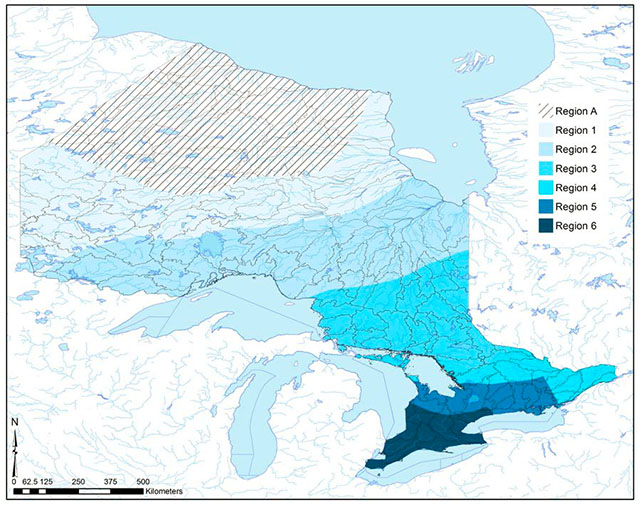
1.1.1. Proration
Prorating streamflow time series from one location to another on the main channel of the same river or from nearby gauged watersheds that are hydrologically similar is a preferred method if data is available. Prorate means to divide or distribute proportionately. In hydrology, proration is used to transfer streamflow time-series from a gauged site to an ungauged site using the ratio of the respective drainage basin areas as a correction factor. For example, daily streamflow at a gauged site with a basin area of 5000 km2 can be used to estimate flows at an ungauged site 10 km upstream with a drainage basin area of 4500 km2 by multiplying the daily flow at the gauged site by 0.9. Thus, direct adjustment of daily streamflow time series data using the ratio of ungauged to gauged drainage basin area as a correction factor is used to simulate flows at the ungauged site. Proration is based on a general assumption frequently made in hydrology that stream discharge and drainage area scale linearly or in a near linear fashion (Dunne and Leopold 1978; Galster et al. 2006; Galster 2007). This method is best applied at sites with drainage areas > 100km2 and where there is not a significant difference (orders of magnitude) between drainage basin areas of the two sites.
Uncertainty in prorated streamflow estimates increases with increasing differences in basin characteristics between the gauged and ungauged sites. In addition to drainage area, many basin characteristics affect a river’s flow regime including basin physiography, stream order, channel morphometics, geology, landcover and land use, in addition to the proximity to the ungauged basin (Maidment 1993). The suitability of transferring streamflow data across drainage basins increases where common characteristics can be identified (Moin and Shaw 1986a, 1986b; Acres International Inc. 1994; OMOE 1995, 2008; OMNR 2000). When significant differences exist, a deterministic rainfall-runoff model developed, calibrated and validated for the gauged site can be used to transfer the time-series to the ungauged site.
1.1.2. Back-calculating natural inflows to reservoirs
In cases where natural flows enter a reservoir, the inflow can be back-calculated using measured outflow from the dam/waterpower facility (m3sec-1) and changes to reservoir storage (m3) over the same time period (t). Outflow can be obtained directly through instrumentation or estimated using stage-discharge curves. Similarly, changes to reservoir storage can be obtained using stage (m) - storage (m3) rating curves based on knowledge of the hypsometric reservoir volume. The magnitude of uncertainty in the estimates would depend on the importance of other physical features governing inputs and outputs to the reservoir (e.g. evaporation, exfiltration, and rainfall interception due to changes in water surface area). However, in most cases, these sometimes offsetting variables will have little influence on the magnitude or pattern of the simulated time series and the procedure can be applied with confidence.
1.1.3. Spatial interpolation
Spatial interpolation and regionalisation methods use available observed streamflow data and their associated flow duration curves (FDCs) to simulate flow regimes for ungauged sites. FDCs show the proportion of time a flow value is equalled or exceeded and, by incorporating the complete range of river flows, provides the most informative summary of a flow regime (Searcy 1959; Vogel and Fennessey 1995). Daily flow simulation methods using spatial interpolation have been the focus of considerable research in South Africa for the specific purpose of conducting in-stream flow assessments (Hughes and Smakhtin 1996; Smakhtin et al. 1997; Smakhtin 1999; Smakhtin and Masse 2000). Results from these studies suggest that spatial interpolation and regionalisation methods using FDCs offer an initial, pragmatic approach for simulating natural flow regimes. A similar method has been employed to assess streamflow at ungauged small-scale waterpower sites in Ontario (Acres International Ltd. 1988a, 1988b). A summary of the spatial interpolation method is provided below. Details of the methodology can be found in Hughes and Smakhtin (1996), Smakhtin et al.(1997), Smakhtin (1999), and Smakthin and Masse (2000).
In essence, the spatial interpolation method assumes that flows occurring simultaneously at sites, which are reasonably close to each other and hydrologically similar, correspond to similar percentage points on their respective FDC’s. Locations requiring a simulated streamflow time series are referred to as destination sites. The gauged locations with available streamflow time series that are used for generating data at ungauged sites are referred to as source sites. These sites should include those known to possess a long-term natural flow hydrograph and be located in the same hydroclimatic region (≈100 km radius or less) of the ungauged basin. Simply, the procedure is to transfer the streamflow time series from the location where the data are available to the location where the time series is needed. The methodology includes three sequential steps: 1) Determination of the regional non-dimensional FDC; 2) Calculation of the actual FDC at the destination site by multiplying the non-dimensional curve by the long-term mean discharge at that site; and 3) Conversion of an actual FDC at a site into a continuous streamflow hydrograph using the spatial interpolation technique.
Step 1: Generation of a regional flow duration curve (FDC)
A representative “regional” FDC is determined by selecting a gauged site with a long- term natural flow regime, which is relatively close to the ungauged site(s) of interest and demonstrates a similar pattern of flow variability. Similarity in flow pattern is assessed using landscape parameters (i.e. percentage of drainage basin covered by lakes and wetlands, or basin shape) upstream of the ungauged and gauged sites as these factors partially determine the hydrologic similarity between the sites. The ordinates of the curve are then standardised by dividing flows from the curve by the gauged long-term mean daily flow.
Alternatively, a few gauged, similar sized catchments with natural flow regimes in the same hydroclimatic region with reliable and unmodified flow records should be identified. Each “gauged” curve is then standardized by the long-term mean discharge, estimated from the observed record, and the average of all curves is calculated. A regional FDC reflects regional flow variability. Averaging of the non-dimensional ordinates of the curves is done for the 17 fixed percentage points (0.01, 0.1, 1, 5, 10, 20, 30, 40, 50, 60, 70, 80, 90, 95, 99, 99.9 and 99.99%). An average of several FDC’s within the same region is more reflective of regional flow variability.
Step 2: Generation of a FDC for the destination site
The next step is to calculate the actual reference FDC for an ungauged WPF site. This is accomplished by multiplying the non-dimensional regional FDC ordinates (standardised flows) by the long-term mean discharge at an ungauged site. Estimates of long-term natural mean annual flow may be obtained using regional estimation methods available in Ontario (OMNR 2000; Acres 1994). These models have been incorporated in the Ontario Flow Assessment Techniques software (Chang et al. 2002). Alternatively, if a representative gauged site is close to the ungauged site of interest and within the same watershed, a FDC at the ungauged site may be established using a correction factor as a ratio of the catchment areas (at the gauged site and at the WPF site). In any case, a FDC is represented by a table of 17 fixed percentage points listed above and their corresponding flows. Each standardized flow is multiplied by the selected correction factor and a table of actual flow values for the fixed percentage points is produced.
Step 3: Generation of a continuous streamflow hydrograph for the destination site
Conversion of the destination site FDC into continuous daily time series is accomplished using the spatial interpolation technique of Hughes and Smakhtin (1996). This is not strictly a modelling technique, as it deals exclusively with already available records. The main assumption of the method is that flows occurring simultaneously at sites in a reasonably close proximity to each other correspond to similar percentage points on their respective FDCs. This implies that the source and destination flow regimes will display a certain degree of similarity in the sequence of flows (i.e. if there is a peak flow at the source site, there is also a high flow at the destination site). This may be ensured if the source sites are selected from within the surrounding area in close proximity to the destination. The degree of similarity between each source site and a destination flow regime site is arbitrary, and can be ranked by assigning a weighting factor to each source site.
If only one source site is used, the core computational procedure for each day includes: i) Identification of the percentage point position of the source site’s streamflow on the source site’s FDC; and ii) Reading off the flow value for the equivalent percentage point from the destination site’s flow duration curve (Figure 2). If more then one source site is used, the two steps above are repeated for each site, resulting in more then one estimate of the destination site flow on the same day (i.e. if two source sites are used, there will be two estimates). The final destination site flow value on each day is estimated as the weighted average of all estimated destination site flow values, repeated for each day.
To generate streamflow time series at a destination site (ungauged site), more than one source site is recommended where possible. The use of several source sites is an attempt to account for the fact that a destination site time series may be the result of several influences, which may not be reflected in a single source site time series. Also, part of an individual source site time series may be missing, therefore, the use of several should decrease the number of missing values in the resultant time series at the destination site.
Additional details about this computational procedure are available from Hughes and Smakhtin (1996) or Smakhtin (2000). Both sources describe a number of case applications of the spatial interpolation approach, illustrate the examples of source site selection, assignment of weighting factors, and examine the implications of both on the destination flow time series.
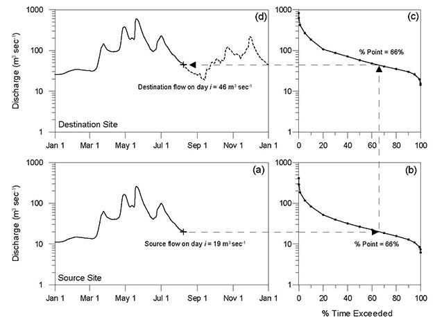
1.1.4. Rainfall-runoff models
Hydrological modelling involves the simplification and conceptual representation of parts of the hydrologic cycle. Hydrological modelling is most often used for hydrologic prediction, including predicting rainfall-runoff relationships in ungauged basins and to enhance understanding of hydrological processes operating within a drainage basin. Improvements in the simulation and prediction of streamflow data in ungauged basins or for the purpose of extending or patching missing data periods may be achieved using hydrological models that simulate rainfall–runoff response over a range of spatial and temporal scales. Generally, hydrologic models can be categorised as being lumped, semi-distributed, or distributed, with increasing data requirements and model parameterisation, respectively.
Lumped hydrologic models use basin average input data to produce total basin streamflow. These models may produce reasonable results but because of the distributed nature of hydrological properties like soil type, slope and land-use, the model cannot be expected to accurately represent the spatial variability in watershed conditions (Flügel and Lüllwitz 1993). Lumped models are widely used because they require fewer input data and pose less burden in computation. Specific examples of these models include the gr2m water balance model (Makhlouf and Michel 1994) and HSPF (Hydrological Simulation Program – Fortran) (Bicknell et al. 1997; EPA 1997).
Distributed hydrologic models have the capability of incorporating a variety of spatially variable data, including remotely sensed data, resulting in simulations that possess higher resolution than lumped models and potentially improving hydrologic predictions (Carpenter and Georgakakos 2006) However, distributed models are generally considered to be limited in their application because of the high costs and data limitations associated with the large volume of data required to run them (Onyando et al. 2003) relative to other hydrological modelling systems. Examples of common distributed models include watflood (Kouwen 1988), mike she (DHI 1998), topmodel (Beven et al. 1984), and PRMS (Precipitation-Runoff Modeling System) (Leavesley et al. 1983). Moving from a lumped to a distributed model structure can significantly increase the number of parameters that must be estimated (Ajami et al. 2004). Thus, it is important to weigh the potential improvement in prediction over lumped models versus the added cost, time and data requirements, increased overall complexity and inherent uncertainty in estimating distributed model parameters (Carpenter and Georgakakos 2004).
Physically-based, semi-distributed hydrologic models account for the spatial distribution of flows through the aggregation of hydrological processes within subunits based on basin characteristics (Onyando et al. 2003). These attributes make the semi-distributed models less complex in comparison to the distributed models, but at the same time maintain the advantages of distributed hydrological information (Onyando et al. 2003). Some commonly used semi-distributed models include the HBV model (Bergström 1976, 1992) and the Soil Water Assessment Tool (SWAT) (Gassman et al. 2007). Input parameters to semi-distributed models can include recorded data on precipitation, air temperature, evapotranspiration, geographical information about the river and catchment and a streamflow record to support model calibration.
Thus, to ensure cost effective and parsimonious modelling of natural flow regimes at ungauged sites with acceptable uncertainty, semi-distributed models, such as HBV, or lumped models are recommended as an alternative when the paucity of gauges prohibits use of the other methods described. More detailed information on the use and application of acceptable continuous simulation models can be found in Section E:2 of OMNR (2002).
1.1.4.1. Hydrologiska Byråns Vattenbalansavdelning (HBV) model
The HBV model, originally developed by SMHI (Swedish Meteorological and Hydrological Institute) in the early 70´s to assist hydropower operations (Bergström, 1976, 1992), is a conceptual rainfall-runoff model that quantifies hydrological processes at the catchment scale. The aim was to create a hydrological model with reasonable demands on computer facilities and calibration data. As such, data input requirements are limited to mean daily temperature and total precipitation and values for a limited number of model parameters. Although originally designed for hydrological forecasting in calibrated basins, applications have expanded to include filling gaps in time series, simulation of streamflow at ungauged sites, design flood calculations and water quality modelling. A version of HBV optimised for conditions in Canada has been developed by the National Research Council’s Canadian Hydraulics Centre (https://www.nrc-cnrc.gc.ca/eng/ibp/chc/software/kenue/green-kenue.html) [link inactive] and another version optimised for conditions in Ontario (MAC-HBV), particularly lowflows, has been developed by McMaster University (Samuel et al. 2010, 2011a; 2011b) . Other information can be obtained from SMHI (http://www.smhi.se/forskning/forskningsomraden/hydrologi/hbv-1.1566) [link inactive].
1.2. Baseflow separation
Baseflow time series are generated using continuous time series of total streamflow and baseflow separation techniques that separate event-based from non event-based water (Smakhtin 2001; Chapman 1999). These baseflow separation techniques divide the streamflow hydrograph into its component parts of baseflow and surface runoff to estimate the groundwater and surface storage contribution to total streamflow (Nathan and McMahon 1990; Chapman 1999; Neff et al. 2005). Because baseflows derived using this technique represent the historic range of baseflow variability for a natural river system over a selected period of record, baseflow is an appropriate measure of low flows and viewed as a useful indicator of the true ecological flow for a river (Smakhtin 2001). An important benefit of this approach over other statistical methods is that it uses well established hydrograph separation techniques and natural flow time-series data to estimate the flow component of interest directly.
Many proven continuous hydrograph-separation algorithms are available for separating baseflow from total flow (Nathan and McMahon 1990; Sloto and Crouse 1996; Chapman 1999; Neff et al. 2005; Piggott et al. 2005; Eckhardt 2008). This includes the bflow filter which uses the digital filter method originally developed by Lyne and Hollick (1979) and the DOS-based bflow filter program developed by Arnold and Allen (1999). The bflow filter requires one filter parameter be defined to support the filtering of high frequency signals. Nathan and McMahon (1990) showed that a filter parameter of 0.925 provided realistic results when compared to manual baseflow separation methods. The method described here follows the procedure of Nathan and McMahon (1990), who found that the use of a recursive digital filter was a fast and objective method of continuous baseflow separation. The justification for the use of this method rests on the fact that filtering out high-frequency signals is intuitively analogous to the separation of low-frequency baseflow from the higher frequencies of quick flow by passing the filter over the streamflow record three consecutive times - forwards, backwards, and forwards again (Nathan and McMahon 1990). The bflow algorithm is:
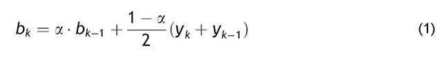
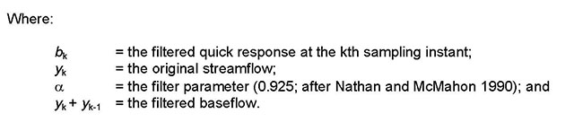
bk = α·bk−1 + [(1−α) ÷ 2] × (yk + yk−1)
Where
- bk = the filtered quick response at the kth sampling instant;
- yk = the original streamflow;
- α = the filter parameter (0.925; after Nathan and McMahon 1990);
- and yk + yk-1 = the filtered baseflow.
A recent study examining baseflow in the Great Lakes Basin identified that the bflow recursive digital filter returned the lowest baseflow values when compared to five of the most commonly used hydrograph separation methods (Neff et al. 2005). Thus, using the bflow algorithm as a basis for calculating baseflow indicators in Ontario basins provides some assurance that indicator values will not be overestimated. Additional research undertaken in Ontario by Metcalfe et al. (2005b) supports the use of bflow as it was shown to produce baseflow values that correlated well with land use and surficial geology in Ontario. It was also found to be the optimum method for baseflow separation for watercourses within the Grand River watershed (unpublished report 2003). These findings suggest that the bflow filter following the procedure of Nathan and McMahon (1990) describes basin hydrology well in Ontario and provides a sound method upon which to calculate baseflow indicators. The bflow algorithm has been included in the Streamflow Analysis and Assessment Software (SAAS).
1.3. Supporting information
1.3.1. Streamflow simulations
The following information is suggested to accompany a streamflow simulation to allow a thorough assessment of the quality of the time series:
- A regional analysis of stream gauges and control structures, including:
- A description of all stream gauges in the area, most often operated by the Water Survey of Canada (WSC).
- A description of existing control structures that may be altering flows observed in the historical streamflow record from gauges identified in (i).
- A map showing the location of stream gauges, control structures and the proposed development site.
- A table that includes: Gauge ID, gauge name, if the gauge is active or decommissioned, river name, period of record, gauge drainage area, and comments on upstream alteration.
- Rationale for the choice of streamgauges used to simulate the flow regime.
- A table showing the gauges selected for the flow simulation that includes: Gauge ID, river name, and details on the use of the gauge (e.g. weighting factors etc.).
- Digital daily mean discharge with associated meta data in the following comma delimited format reported to two significant digits:
- Site name,
- Site ID,
- Easting,
- Northing,
- Start date,time
- End date,time
- Day/month/year,daily mean discharge (m3sec-1)
For example,
- Ontario gs
- 5BD60
- 340340
- 5305305
- 31/12/2008
- 04/01/2009
- 31/12/2008,40.17
- 01/01/2009,40.17
- 02/01/2009,40.33
- 03/01/2009,40.44
- 04/01/2009,40.55
….etc
- If using the HBV or similar hydrological model to simulate the flow regime:
- Model parameters and associated values;
- Value for NVE (Nash-Volume Error Efficiency) for the calibration;
- Sqrt NSE (indication of model performance for peak flows);
- Log NSE (indication of model performance for low flows);
- Associated thresholds (outside of which model results are difficult to use); and
- Absolute volume error (AVE) – catchment based.
2. Field-based assessments
2.1. Hydrometric field techniques
The purpose of the hydrometric monitoring is to improve flow simulations and increase the accuracy of indicator and assessment criteria values. Data collected from the site can be correlated with historical flow records used in proration and spatial interpolation methods or for validating/optimising a hydrologic model. Significant improvements will be observed when the monitoring period captures the full distribution of flows observed at the site, achieved by monitoring for a minimum of 12 months but the best results will be obtained with longer monitoring programs that capture inter-annual variability.
The development of a new hydrometric station combined with the short monitoring period will require an intensive sampling program for discharge measurements to adequately establish a stage-discharge relation over the greatest range of stage possible. More frequent sampling should be conducted during high and low magnitude flows to increase certainty in the tails of the curve. The timing of high and low flows can be estimated by historical flow records from nearby stream gauges to assist in the planning of site visits.
Established standards (see below) should be followed to conduct hydrometric surveys and streamflow monitoring as part of the field-based assessment. Each site will present its own challenges; however, the established standards provide flexibility to address site specific challenges while still meeting information requirements.
- Proper site selection, demarcation, installation, maintenance, and operation of a hydrometric station (CAN/CGSB-157.3-M91;CAN/CGSB-157.2-M91).
- Hourly instantaneous recording of water depth (referenced to the deepest location of the cross section) with 2 mm gauge accuracy
- The computation of instantaneous discharge using velocity-area methods (CAN/CGSB-157.2-M91) and/or acoustic Doppler profilers (ISO/TS 24154:2005) and associated measures of uncertainty (CAN/CGSB-157.6-M91).
- The determination of the stage-discharge relation for the site and a measure of uncertainty in the relation (CAN/CGSB-157.4-M91)
- An extension of the rating curve using a log-log plot, if no discharge measurements taken at the highest and lowest observed stage, confirmed with discharge estimates using the slope-area method (ISO 1070:1992). At a minimum, this should be used to estimate bankfull magnitude if not measured directly during the monitoring period.
- The conversion of the instantaneous water level time series into discharge using the rating relation and a mean daily discharge time series computed
- Use of standard terminology and symbols (CAN/CGSB-157.1-M91)
Accepted standards referenced above produced by the Standards Council of Canada include:
- CAN/CGSB-157.3-M91 Liquid Flow Measurement in Open Channels - Establishment and Operation of a Gauging Station
- CAN/CGSB-157.2-M91 Liquid Flow Measurement in Open Channels - Velocity-Area Methods
- CAN/CGSB-157.4-M91 Liquid Flow Measurement in Open Channels - Part 2: Determination of the Stage-Discharge Relation
- CAN/CGSB-157.6-M91 Liquid Flow Measurement in Open Channels - Velocity-Area Methods - Collection and Processing of Data for Determination of Errors in Measurement
- CAN/CGSB-157.1-M91 Liquid Flow Measurement in Open Channels - Vocabulary and Symbols
- Accepted standards referenced above produced by International Organisation for Standardization (ISO) include:
- iso/ts 24154:2005 Hydrometry – Measuring river velocity and discharge with acoustic Doppler profilers
- iso 1070:1992 Liquid flow measurement in open channels - Slope-area method
2.2. Determining bankfull stage
Field measurement of bankfull flow magnitude requires: i) the physical identification of bankfull stage in the field; and ii) calculation of bankfull discharge associated with the stage measured in (i). Once the bankfull discharge is known, the recurrence interval is determined using flood frequency analysis and the streamflow time series analysed to characterise the timing and duration of flows of this magnitude.
Step 1: determining bankfull stage
Standardized field methods to determine the magnitude of bankfull flows (e.g. either channel cross-sectional measurements or direct observation of flows at a variety of discharges) combined with a characterisation of those flows based on the natural flow record, provides a physically-based, well-founded method for making environmental flow recommendations (Tharme 1996). Stanfield et al. (1999) discuss methods to measure bankfull stage in the field. They suggest using cross-sections void of obscuring features such as: i) large woody debris in the channel or on the banks; ii) inorganic deflectors such as mid-channel islands and large boulders; iii) bank armour, such as rip rap, gabion, or concrete; iv) bank failures; v) trampled banks; or vi) proximity to tributaries or outlets. Suggested methods to measure bankfull stage using different features in the channel’s cross-section and an indication of their reliability are shown in Table 1.
For cross-sections where bankfull stage is not easily defined using the indicators described above, ratios of channel width to channel depth can be calculated (Figure 3). The river stage that gives the lowest value for the width/depth ratio is considered to best indicate bankfull stage (Wolman 1955; Knighton 1998).
| Method | Reliability | Comments |
|---|---|---|
| 1. Floodplain elevation | High | Bankfull stage is equal to the height of the floodplain in rivers or streams with a defined floodplain. |
| 2. Inflection points | High | Stream bed and bank erosion occurs with increasing discharge and produces breaks in the bank profile which can indicate bankfull stage. Multiple inflection points are common; where vegetation is sparse this may be the best indication of bankfull stage. |
| 3. Changes in bank material | Medium- high | The change from a finer bank material to a coarser bank material can be an indicator of bankfull stage, but parent (underlying) material must be considered. The bank material transition may also be from cohesive to non-cohesive, or organic to inorganic. |
| 4. Changes in vegetation | Medium | Most plant (especially the roots of trees and shrubs) are either water tolerant or intolerant, and bankfull stage may be indicated by rooting elevation. Depth of root penetration into a bank may also be an indicator. Certain species thrive just above bankfull stage. |
| 5. Maximum point bar elevation | Medium-low | Point bars are morphologic features adjacent to scour pools at a meander bend, and they are usually just submerged at bankfull flow. This level may also be associated with an inflection point on the river bank adjacent to the scour pool. |
| 6. Presence of thatch, water stains, burrows, or nests | Low | Thatch (debris, grass) and water stains can provide an indicator of recent flow level, but this may not be indicative of bankfull stage. Animals tend to burrow or nest just above the bankfull stage. |
Step 2: Calculating bankfull discharge
Once bankfull stage has been determined in the field, bankfull discharge can be estimated by measuring flow velocities and channel cross-sectional area at bankfull. However, the duration of bankfull discharge, combined with safety issues related to taking such measurements at high flows, limits the opportunities to obtain actual field measurements of a bankfull event. In the absence of field measurements, bankfull discharge can be estimated using rating curves and flow modelling.
It is easiest to estimate bankfull stage at sites close to established stream flow gauging stations since the historical flow record and rating curve from the gauging station can be used to estimate bankfull discharge. Rating curves for Water Survey of Canada (WSC) stream gauges are available from the nearest regional office. One difficulty with this method is that bankfull stage measurement in the field is not always transferable to a corresponding gauging station’s rating curve, as many stations use stilling wells that are not always calibrated to the stream channel bed (depth = 0m), thus a correction factor is required in these instances.
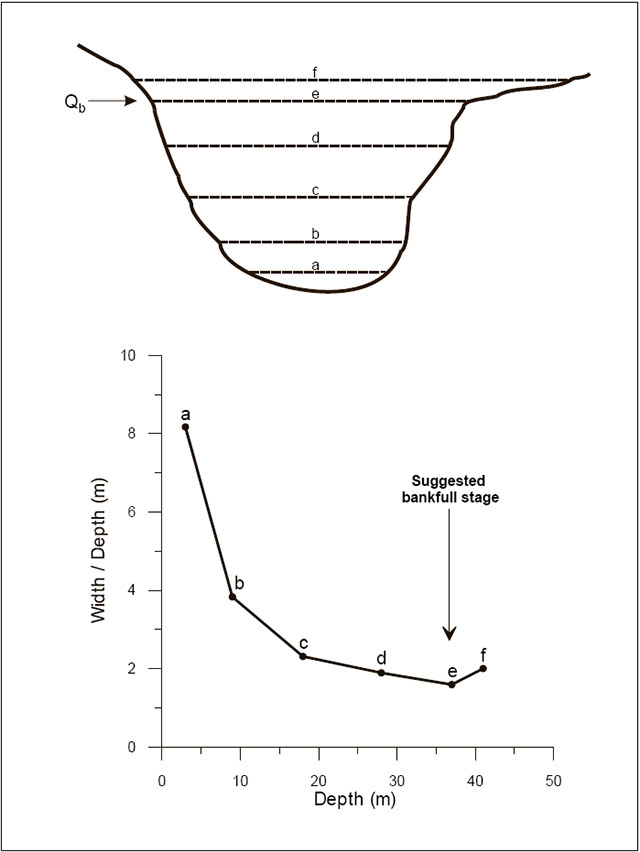
Estimates of bankfull discharge can also be modelled using the slope-area method and measured channel parameters. Typically, the Gauckler-Manning flow equation (Schumm 1960; Pickup and Warner 1976; Radecki-Pawlik 2002) is used to calculate bankfull discharge (Qb):

Qb = (1 ÷ n)AbDb2/3S1/2
where n is the resistance coefficient (Manning’s ‘n’), Ab is the bankfull discharge cross-sectional area (m2), Db is the bankfull depth (m), and S is the river channel slope. Manning’s ‘n’ is a roughness coefficient, that can be calculated empirically:
v = (R2/3 s1/2) ÷ n
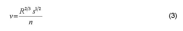
where v is mean velocity, R is hydraulic radius, and s is slope of the energy gradient. Manning’s n can also be estimated from descriptions of river channels and river channel character, or from many published sources (e.g. Barnes Jr. 1967; Selby 1985; Acrement and Schneider 1989; Sanders 1998).
Various flow modeling software packages are available that use these channel parameters obtained through field measurement to estimate discharges for increasing flow stage. For example, Winxspro (Grant et al. 1992) requires information on cross- channel geometry, channel bed slope, water surface slope, and bed roughness to estimate discharge. Bankfull flow stage can be input as maximum flow depth to estimate bankfull discharge.
An estimate of bankfull discharge using the slope-area method should be an average based on at least three different cross-sections to reduce uncertainty in the estimate.
2.3. Supporting information
2.3.1. Streamflow
The following information is suggested to accompany a streamflow simulation refined through hydrometric monitoring to allow an assessment of the quality of the time series:
- A description, photographs, and UTM coordinates for the site.
- A detailed cross-sectional profile for streamflow sites (see chapter on Sediment Regime).
- A detailed list of equipment used for the hydrometric station and technical specifications.
- Chronological summary of gauge level checks with all corrections identified.
- A fully documented methodology for discharge measurements and rating curve development,
- Rating curve(s)
- Consisting of a minimum of 10 discharge measurements distributed through the range of flows but with particularly good coverage at the low and high magnitudes plotted with dates of measurement.
- Point symbols to denote whether discharges were measured or estimated (i.e. using the slope area method).
- Individual curves identified with the period of use, if applicable.
- Equation for rating relation and correlation coefficient
- A spreadsheet summary showing date, stage, measured discharge, estimated discharge
- FDC for the monitoring period.
- Digital hourly instantaneous stage, discharge and computed daily mean discharge with associated meta data in the following comma delimited format reported to two significant digits and missing data identified as -999:
- Site name, Site ID, Easting, Northing,
- Start date,time
- End date,time
- Day/month/year,hr:min,stage (m),hourly discharge (m3sec-1), daily mean discharge (m3sec-1)
For example,
- Ontario GS
- 5BD60
- 340340
- 5305305
- 01/01/2008,24:00
- 01/01/2009,24:00
- 31/12/2008,24:00,124.37,40.17
- 01/01/2009,01:00,124.37,40.17
- 01/01/2009,02:00,124.38,40.33
- 01/01/2009,03:00,124.39,40.44
- 01/01/2009,04:00,124.40,40.55
- 01/01/2009,24:00,124.37,40.17,40.53
- An updated flow simulation and model outputs (if appropriate).
2.3.2. Bankfull flow
The following information should accompany field estimates of bankfull flow to allow an assessment of the quality of the estimate:
- A description, photographs, and UTM coordinates for the site(s).
- A rating curve with rating relation, correlation coefficient, and stage depth clearly marked; or
- Detailed cross-sectional profile (3 if using the slope-area method).
- Values for bankfull width, depth, cross-sectional area.
- Values for model parameters if using the slope area method.
3. Monitoring
The goal of hydrometric monitoring is to adequately represent the pattern and magnitude of water level fluctuation and in the case of rivers, convert water levels to flow using discharge rating curves. Like all environmental monitoring of continuously changing variables, this is achieved by determining the optimum time interval to record an observation to fully represent the pattern of change while minimising the loss of information and data storage requirements.
Observations can be recorded instantaneously or can be a statistic that integrates instantaneous observations over a set time interval. Thus, it is important to differentiate between the data sampling interval and the data logging interval.
Data sampling interval: Interval at which water levels are sampled instantaneously (e.g. 5, 15, 60 minute).
Data logging interval: Interval at which water levels (instantaneous or summary statistic) are recorded (e.g. daily average discharge)
3.1. Practices/standards at the Water Survey of Canada
Canada’s hydrometric network, overseen by the Water Survey (WSC) in partnership with the provinces and territories, is the most common source of surface water quantity data in Canada. As a minimum requirement, all water sensors employed by the WSC must be capable of sampling water levels every 5 minutes. This five minute sample set may be from an instantaneous single sensor reading or an average of instantaneous sensor readings taken over an ‘integration period between a minimum of 5 seconds and a maximum of 120 seconds. These readings become the sample set from which the maximum and minimum instantaneous values are derived for a set period (usually 24 hours). For logging, the minimum standard requires that one instantaneous water level reading per hour be recorded, on the top of the hour, and at least one maximum and one minimum 5-minute instantaneous reading per day be recorded. This standard is thought to provide an accurate representation of river behaviour without creating large volumes of data. Both sampling and logging frequency described is a minimum requirement but can be increased to address site specific operational considerations.
3.2. Data resolution and streamflow pattern
Although publicly distributed at daily time intervals, collection of data adhering to the standards outlined above is available on request. Hourly instantaneous discharge data obtained from the Water Survey for existing stream gauges downstream of waterpower facilities is shown in Figure 4. The hydrographs from each gauge using the 60-minute data sampling interval show clear indications of an altered streamflow pattern. Also demonstrated is the loss of this information at the 24-hour interval using either instantaneous or averaged daily discharge values. An examination of data loss over finer data sampling intervals is examined in Figure 5 using instantaneous discharge data observed at a research site downstream of a peaking waterpower facility. Although there appears to be little information loss moving from the 15-minute to the 60-minute data sampling interval, the inadequacy of a 24-hour data sampling interval to represent the altered flow pattern is again apparent. However, the rate-of-change of flow calculated for this same time period and intervals does highlight differences even at the finer sampling intervals (Figure 6). The ‘smoothing’ effect occurs with increasing time interval, evidenced in the time series plots and the decrease in the mean and maximum rate of change.
Hydrometric monitoring must be of sufficient temporal resolution as to advance ones understanding of aquatic ecosystem response to hydrologic alteration. It is clear that a 24-hour sampling interval (i.e. daily discharge) is not adequate to represent the true pattern of an altered flow regime. The 60-minute sampling interval, adopted by the Water Survey of Canada, as a minimum reporting standard, would appear to adequately describe streamflow pattern on some altered systems. However, this sampling interval may not be adequate for altered systems that are more responsive. These systems can be likened to that of small bedrock basins and urban environments. In these instances, both the Water Survey of Canada and the U.S. Geological Survey have found it necessary to use shorter sampling intervals to adequately capture the rate-of-change of flow and thus streamflow pattern. Similarly, 15 minute intervals are preferred for altered systems in British Columbia (LWBC 2005). Thus, on some altered systems, shorter sampling intervals may be required to represent the true pattern of flow.
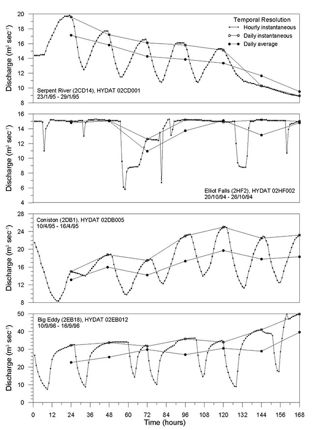
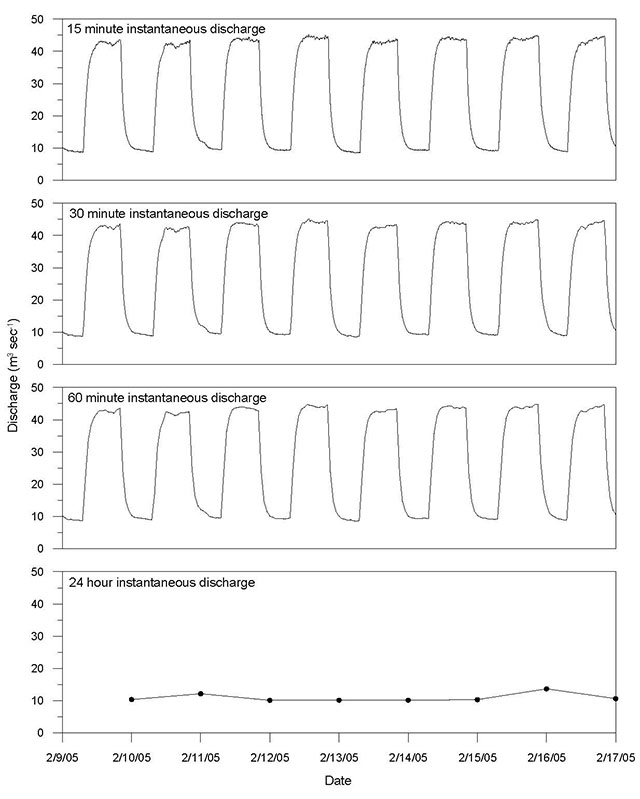
3.3. Supporting information
Hydrological data collected as part of a monitoring program to adequately assess hydrologic alteration should include:
- A minimum of an instantaneous discharge reading per hour be recorded, on the top of the hour;
- On systems with higher rates of change of flow and more erratic flow patterns that it be determined if shorter sampling intervals are required to represent better the rate of change of flow and resulting flow pattern;
- Data requirements for reservoir water levels that match those for flows; and
- Data assessed on an annual basis using the comma delimited format (a common standard output of all database and analysis software) shown below. Each file should begin with the required metadata followed by the time series information. Flow and level data should be reported to two significant digits.
- Site name,
- Site ID,
- Easting,
- Northing,
- Start date, time
- End date,time
- Day/month/year,hr:min, power flow(cms), spill flow(cms), headpond water level(m)
For example,
- Ontario GS
- 5bd60
- 340340
- 5305305
- 01/01/2006,01:00
- 01/01/2006,04:00
- 01/01/200601:00,40.17,0.00,124.37
- 01/01/2006,02:00,40.33,0.00,124.35
- 01/01/2006,03:00,40.44,0.00,124.33
- 01/01/2006,04:00,40.55,0.00,124.23
Addendum I: Possible steamgauges suitable for establishing reference conditions in ungauged basins
| Station Number | Station Name | Area km2 | Flow Status | Operational Status | Tertiary Basin | Major Basin | Record Start Date | Record End Date | Latitude | Longitude | Additional Info | |
|---|---|---|---|---|---|---|---|---|---|---|---|---|
| 02AB008 | Neebing River near Thunder Bay | 187 | N* | A₪ | 2AB | Lake Superior | 1953 | 48°23′0″ | 89°18′23″ | |||
| 02AB017 | Whitefish River at Nolalu | 210 | N | A | 2AB | Lake Superior | 1980 | 48°17′31″ | 89°48′35″ | |||
| 02AC001 | Wolf River at Highway no. 17 | 736 | N | A | 2AC | Lake Superior | 1971 | 48°49′18″ | 88°32′4″ | |||
| 02AD010 | Blackwater River at Beardmore | 650 | N | A | 2AD | Lake Superior | 1971 | 49°35′51″ | 87°57′55″ | |||
| 02AE001 | Gravel River near Cavers | 616 | N | A (D)^ | 2AE | Lake Superior | 1974 | 48°55′33″ | 87°41′24″ | Missing data between 1995-2005 (Station was Discontinued) | ||
| 02BA002 | Steel River near Terrace Bay | 1190 | N | D‡ | 2BA | Lake Superior | 1970 | 1994 | 48°46′40″ | 86°53′4″ | Replaced with 02BA006 further upstream on Steel River | |
| 02BA003 | Little Pic River near Coldwell | 1320 | N | A | 2BA | Lake Superior | 1972 | 48°50′56″ | 86°36′25″ | |||
| 02BA006 | Steel River below Santoy Lake | N/A∞ | N | A | 2BA | Lake Superior | 2003 | 48°48′49″ | 86°51′33″ | |||
| 02BB003 | Pic River near Marathon | 4270 | N | A | 2BB | Lake Superior | 1970 | 48°46′26″ | 86°17′47″ | |||
| 02BD003 | Magpie River near Michipicoten | 1930 | N | D | 2BD | Lake Superior | 1939 | 1990 | 47°56′20″ | 84°49′50″ | Discontinued, but serves as useful indicator of natural flow in the area | |
| 02BF001 | Batchawana River near Batchawana | 1190 | N | A | 2BF | Lake Superior | 1967 | 47°0′12″ | 84°30′56″ | |||
| 02BF002 | Goulais River near Searchmont | 1160 | N | A | 2BF | Lake Superior | 1967 | 46°51′39″ | 83°58′18″ | |||
| 02CA002 | Root River at Sault Ste. Marie | 108 | N | A | 2CA | Lake Huron | 1971 | 46°33′46″ | 84°16′54″ | |||
| 02CB003 | Aubinadong River above Sesabic Creek | 1440 | N | A | 2CB | Lake Huron | 1980 | 46°58′6″ | 83°25′0″ | |||
| 02CF007 | Whitson River at Chelmsford | 243 | N | A | 2CF | Lake Huron | 1960 | 46°34′58″ | 81°11′57″ | |||
| 02CF008 | Whitson River at Val Caron | 179 | N | A | 2CF | Lake Huron | 1960 | 46°36′36″ | 81°1′58″ | |||
| 02DC004 | Sturgeon River near Glen Afton | 2980 | R** | A | 2DC | Lake Huron | 1941 | 46°38′13″ | 80°15′47″ | Designated as ‘Regulated’ by WSC but has natural flow pattern | ||
| 02DC012 | Sturgeon River at Upper Goose Falls | 1200 | N | A | 2DC | Lake Huron | 1986 | 46°58′17″ | 80°27′47″ | |||
| 02DD012 | Veuve River near Verner | 741 | N | A (D) | 2DD | Lake Huron | 1973 | 2010 | 46°24′29″ | 80°7′23″ | Missing data between 1993-2009 (Station was Discontinued) | |
| 02DD015 | Commanda Creek near Commanda | 106 | N | A | 2DD | Lake Huron | 1974 | 45°56′57″ | 79°36′24″ | |||
| 02EA005 | North Magnetawan River near Burk’s Falls | 321 | N | A | 2EA | Lake Huron | 1915 | 2010 | 45°40′10″ | 79°22′45″ | ||
| 02EA010 | North Magnetawan River above Pickerel Lake | 149 | N | A | 2EA | Lake Huron | 1968 | 45°42′13″ | 79°18′31″ | |||
| 02EC002 | Black River near Washago | 1520 | N | A | 2EC | Lake Huron | 1915 | 44°42′49″ | 79°16′53″ | |||
| 02HD012 | Ganaraska River above Dale | 232 | N | A | 2HD | Lake Ontario | 1976 | 43°59′27″ | 78°19′41″ | |||
| 02HL004 | Skootamatta River near Actinolite | 712 | N | A | 2HL | Lake Ontario | 1955 | 44°32′58″ | 77°19′41″ | |||
| 02JC008 | Blanche River above Englehart | 1780 | N | A | 2JC | Ottawa River | 1968 | 47°53′20″ | 79°52′45″ | Recent Data (2009) shows regulation during low flows (from Misema GS) | ||
| 02KB001 | Petawawa River near Petawawa | 4120 | R | A | 2KB | Ottawa River | 1915 | 45°53′10″ | 77°18′55″ | Designated as ‘Regulated’ by WSC but has natural flow pattern; RHBN Station | ||
| 02KF011 | Carp River near Kinburn | 269 | N | A | 2KF | Ottawa River | 1971 | 45°14′57″ | 75°47′26″ | |||
| 02LB008 | Bear Brook near Bourget | 440 | N | A | 2LB | Ottawa River | 1949 | 45°25′33″ | 75°9′11″ | |||
| 04CA002 | Severn River at Outlet Of Muskrat Dam Lake | 36500 | N | A | 4CA | Severn River | 1965 | 53°29′22″ | 91°30′36″ | |||
| 04DA001 | Pipestone River at Karl Lake | 5960 | N | A | 4DA | Winisk River | 1966 | 52°34′50″ | 90°11′12″ | |||
| 04DB001 | Asheweig River at Straight Lake | 7950 | N | A | 4DB | Winisk River | 1966 | 53°42′42″ | 87°57′12″ | |||
| 04DC001 | Winisk River below Asheweig River Tributary | 50000 | N | A | 4DC | Winisk River | 1965 | 54°29′58″ | 87°13′39″ | |||
| 04DC002 | Shamattawa River at Outlet of Shamattawa Lake | 4710 | N | A | 4DC | Winisk River | 1966 | 54°17′23″ | 85°39′5″ | |||
| 04FC001 | Attawapiskat River below Muketei River | 36000 | N | A | 4FC | Attawap iskat River | 1968 | 53°5′28″ | 85°4′20″ | |||
| 04GA002 | Cat River below Wesleyan Lake | 5390 | N | A | 4GA | Albany River | 1970 | 51°10′25″ | 91°35′40″ | |||
| 04GB004 | Ogoki River above Whiteclay Lake | 11200 | N | A | 4GB | Albany River | 1971 | 50°52′6″ | 88°55′53″ | |||
| 04GB005 | Brightsand River at Moberley | 1170 | N | A (D) | 4GB | Albany River | 1968 | 49°37′25″ | 90°34′19″ | Missing data between 1994-2007 (Station was Discontinued) | ||
| 04JC002 | Nagagami River at highway no.11 | 2410 | N | A | 4JC | Albany River | 1950 | 49°46′22″ | 84°32′13″ | |||
| 04JD005 | Pagwachuan River at highway no. 11 | 2020 | N | A | 4JD | Albany River | 1968 | 49°45′51″ | 85°13′34″ | |||
| 04KA001 | Kwataboahegan River near the Mouth | 4250 | N | A | 4KA | Moose River | 1967 | 51°9′39″ | 80°51′50″ | |||
| 04LJ001 | Missinaibi River at Mattice | 8940 | N | A | 4LJ | Moose River | 1920 | 49°36′50″ | 83°16′0″ | |||
| 04LM001 | Missinaibi River below Waboose River | 22900 | N | A | 4LM | Moose River | 1972 | 50°35′7″ | 82°5′27″ | |||
| 04MD004 | Porcupine River at Hoyle | 401 | N | A | 4MD | Moose River | 1977 | 48°33′0″ | 81°3′15″ | Missing data between 1994-2008 (Station was Discontinued) | ||
| 04MF001 | North French River near the mouth | 6680 | N | A | 4MF | Moose River | 1966 | 51°4′36″ | 80°45′50″ | |||
| 05PA006 | Namakan River at Outlet Of Lac La Croix | 13400 | N | A | 5PA | Nelson River | 1921 | 48°22′57″ | 92°10′34″ | |||
| 05PB014 | Turtle River near Mine Centre | 4870 | N | A | 5PB | Nelson River | 1914 | 48°51′0″ | 92°43′25″ | |||
| 05PB018 | Atikokan River at Atikokan | 332 | N | A | 5PB | Nelson River | 1978 | 48°45′7″ | 91°35′2″ | |||
| 05QA002 | English River at Umfreville | 6230 | N | A | 5QA | Nelson River | 1921 | 49°52′24″ | 91°27′35″ | |||
| 05QA004 | Sturgeon River at Mcdougall Mills | 4450 | N | A | 5QA | Nelson River | 1961 | 50°10′2″ | 91°32′26″ | |||
| 05QC003 | Troutlake River above Big Falls | 2370 | N | A | 5QC | Nelson River | 1970 | 50°54′20″ | 93°5′30″ | |||
| 05QE008 | Cedar River below Wabaskang Lake | 1690 | N | A | 5QE | Nelson River | 1970 | 50°30′27″ | 93°15′30″ | |||
| 05QE009 | Sturgeon River at outlet of Salvesen Lake | 1530 | N | A | 5QE | Nelson River | 1960 | 50°21′08″ | 94° 27′ 59″ | |||
| 05QE012 | Long-Legged River below Long-Legged Lake | 548 | N | A | 5QE | Nelson River | 1980 | 50°40′37″ | 93°58′12″ |
Addendum II: Hydrologic regime assessment table
| Baseflow indicators | Reference condition characterisation % exceed. (m3sec-1 13th 38th 62nd 87th | Current condition if already altered (i.e. not natural) Established baseflow requirement (m3sec-1) | Current condition if already altered (i.e. not natural) % exceed. (if no baseflow requirement) (m3sec-1) 13th 38th Meidan 62nd 87th | Expected condition with new development Expected Baseflow (m3sec-1) | Degree of alteration: current condition (i.e. from reference condition) Low flow magnitude within 38th - 62nd % exceed. | Degree of alteration: current condition (i.e. from reference condition) Medium magnitude between 87th– 62nd or 38th – 13th % exceed. | Degree of alteration: current condition (i.e. from reference condition) High flow magnitude < 13th or > 87th % exceed. | Degree of alteration: proposed condition (i.e. from reference condition) Low flow magnitude within 38th - 62nd % exceed. | Degree of alteration: proposed condition (i.e. from reference condition) Medium flow magnitude between 87th– 62nd or 38th – 13th % exceed. | Degree of alteration: proposed condition (i.e. from reference condition) High flow magnitude < 13th or > 87th % exceed. |
|---|---|---|---|---|---|---|---|---|---|---|
| January | ||||||||||
| February | ||||||||||
| March | ||||||||||
| April | ||||||||||
| May | ||||||||||
| June | ||||||||||
| July | ||||||||||
| August | ||||||||||
| September | ||||||||||
| October | ||||||||||
| November | ||||||||||
| December |
| Subsistence flow indicators | 95th % exceed. (m3sec-1) | 99th% exceed. (m3sec-1) | Established flow requirement for bypassed natural channel reaches (m3sec-1) | Estimated/measured median flow for bypassed natural channel reaches if no requirement (m3sec-1) | Expected flow for bypassed natural channel reach (m3sec-1) | Flow magnitude > 95th % exceed. | Flow magnitude > 99th% exceed. | Flow magnitude < 99th% exceed. | Flow magnitude > 95th % exceed. | Flow magnitude > 99th% exceed. | Flow magnitude < 99th% exceed. |
|---|---|---|---|---|---|---|---|---|---|---|---|
| January | |||||||||||
| February | |||||||||||
| March | |||||||||||
| April | |||||||||||
| May | |||||||||||
| June | |||||||||||
| July | |||||||||||
| August | |||||||||||
| September | |||||||||||
| October | |||||||||||
| November | |||||||||||
| December |
| Subsistence flow indicators | Flow magnitude that covers ≥ 50% of the wetted perimeter for rivers <15m wide and ≥ 70% for rivers > 15 m wide (m3sec-1) | Established flow requirement for bypassed natural channel reaches (m3sec-1) | Estimated/measured median flow for bypassed natural channel reaches if no requirement (m3sec-1) | Expected flow for bypassed natural channel reach (m3sec-1) | Flow magnitude covers ≥ 50% of the wetted perimeter for rivers <15m wide and ≥70% for rivers > 15 m wide | Flow magnitude covers < 50% of the wetted perimeter for rivers <15 m wide and <70% for rivers > 15 m wide | Flow magnitude covers ≥ 50% of the wetted perimeter for rivers <15 m wide and ≥70% for rivers > 15 m wide | Flow magnitude covers < 50% of the wetted perimeter for rivers <15 m wide and <70% for rivers > 15 m wide |
|---|---|---|---|---|---|---|---|---|
| January | ||||||||
| February | ||||||||
| March | ||||||||
| April | ||||||||
| May | ||||||||
| June | ||||||||
| July | ||||||||
| August | ||||||||
| September | ||||||||
| October | ||||||||
| November | ||||||||
| December |
| Rates of change indicators | Percentile (m3sec-1hr-1) 13th, 38th, 62nd, 87th | Percentile (m3sec-1hr-1) 13th, 38th, Median, 62nd, 87th | Expected ROC (m3sec-1hr-1) | ROC within 38th - 62nd percentile | ROC between 13th - 38th, 62nd - 87th percentiles. | ROC < 13th or > 87th percentile. | ROC within 38th - 62nd percentile | ROC between 13th - 38th, 62nd - 87th percentiles. | ROC < 13th or > 87th percentile. |
|---|---|---|---|---|---|---|---|---|---|
| January | |||||||||
| February | |||||||||
| March | |||||||||
| April | |||||||||
| May | |||||||||
| June | |||||||||
| July | |||||||||
| August | |||||||||
| September | |||||||||
| October | |||||||||
| November | |||||||||
| December |
| Frequency indicators | Percentile (frequency) 13th, 38th, 62nd, 87th | Percentile (frequency) 13th, 38th, Median, 62nd, 87th | Expected high flow pulse frequency (frequency) | Frequency within 38th - 62nd percentile | Frequency between 13th - 38th, 62nd - 87th percentiles. | Frequency < 13th or > 87th percentile. | Frequency within 38th - 62nd percentile | Frequency between 13th - 38th, 62nd - 87th percentiles. | Frequency < 13th or > 87th percentile. |
|---|---|---|---|---|---|---|---|---|---|
| Annual | |||||||||
| January | |||||||||
| February | |||||||||
| March | |||||||||
| April | |||||||||
| May | |||||||||
| June | |||||||||
| July | |||||||||
| August | |||||||||
| September | |||||||||
| October | |||||||||
| November | |||||||||
| December |
| Duration indicators | Percentile (days) 13th, 38th, 62nd, 87th | Percentile (days) 13th, 38th, Median, 62nd, 87th | Expected high flow pulse duration (days) | Duration within 38th - 62nd percentile | Duration between 13th - 38th, 62nd - 87th percentiles. | Duration < 13th or > 87th percentile. | Duration within 38th - 62nd percentile | Duration between 13th - 38th, 62nd - 87th percentiles | Duration < 13th or > 87th percentile |
|---|---|---|---|---|---|---|---|---|---|
| Annual | |||||||||
| January | |||||||||
| February | |||||||||
| March | |||||||||
| April | |||||||||
| May | |||||||||
| June | |||||||||
| July | |||||||||
| August | |||||||||
| September | |||||||||
| October | |||||||||
| November | |||||||||
| December |
| Magnitude indicators | Flow magnitude (m3sec-1) | 80% of flow magnitude (m3sec-1) | Flow magnitude (m3sec-1) | 80% of flow magnitude (m3sec-1) | ≥ the 1:1.5 recurrence interval flow magnitude | ≥ 80% of the 1:1.5 recurrence interval low magnitude | < 80% of the 1:1.5 recurrence interval flow magnitude | ≥ the 1:1.5 recurrence interval flow magnitude | ≥ 80% of the 1:1.5 recurrence interval low magnitude | < 80% of the 1:1.5 recurrence interval flow magnitude |
|---|---|---|---|---|---|---|---|---|---|---|
| Preliminary assessment - 1:1.5 recurrence interval flow | ||||||||||
| Field-based assessment - Field estimate of bankfull discharge |
| Duration indicators | Percentile (days) 13th, 38th, 62nd, 87th | Percentile (days) 13th, 38th, Median, 62nd, 87th | Duration within 38th - 62nd percentile | Duration between 13th - 38th, 62nd - 87th percentiles | Duration < 13th or > 87th percentile | Duration within 38th - 62nd percentile | Duration between 13th - 38th, 62nd - 87th percentiles | Duration < 13th or > 87th percentile |
|---|---|---|---|---|---|---|---|---|
| Preliminary assessment - 1:1.5 recurrence interval flow | ||||||||
| Field-based assessment - Field estimate of bankfull discharge |
| Timing indicators | Modal month | Modal month ±1 month | Modal month | Modal month ±1 month | Within modal month | Within 1 month of modal month | Beyond 1 month of modal month | Within modal month | Within 1 month of modal month | Beyond 1 month of modal month |
|---|---|---|---|---|---|---|---|---|---|---|
| Preliminary assessment - 1:1.5 recurrence interval flow | ||||||||||
| Field-based assessment Field estimate of bankfull discharge |
| Magnitude indicators | Flow magnitude (m3sec-1) | Flow magnitude (m3sec-1) | ≥ the associated recurrence interval flow magnitude | < the associated recurrence interval flow magnitude | ≥ the associated recurrence interval flow magnitude | < the associated recurrence interval flow magnitude |
|---|---|---|---|---|---|---|
| 1:2 recurrence interval flow | ||||||
| 1:10 recurrence interval flow | ||||||
| 1:20 recurrence interval flow |
| Duration indicators | Percentile (days) | Percentile (days) | Duration within 38th - 62nd percentile | Duration between 13th - 38th, 62nd - 87th percentiles. | Duration < 13th or > 87th percentile. | Duration within 38th - 62nd percentile | Duration between 13th - 38th, 62nd - 87th percentiles. | Duration < 13th or > 87th percentile. |
|---|---|---|---|---|---|---|---|---|
| 1:2 rcurrence interval flow | ||||||||
| 1:10 recurrence interval flow | ||||||||
| 1:20 recurrence interval flow |
| Timing indicators | Modal month | Modal month ±1 month | Modal month | Modal month ±1 month | Within modal month | Within 1 month of modal month | Beyond 1 month of modal month | Within modal month | Within 1 month of modal month | Beyond 1 month of modal month |
|---|---|---|---|---|---|---|---|---|---|---|
| 1:2 recurrence interval flow | ||||||||||
| 1:10 recurrence interval flow | ||||||||||
| 1:20 recurrence interval flow |
Chapter 3: Sediment regime
List of acronyms
- DEM
- Digital Elevation Model
- HYDAT
- Hydrometric Database for Canada
- MRV
- Maximum reservoir volume
- OSAP
- Ontario Stream Assessment Protocol
- QMAF
- Mean annual streamflow
- TE
- Trap efficiency
- OBM
- Ontario Base Map
- PWQMN
- Provincial Water Quality Monitoring Network
- WSC
- Water Survey of Canada
1.0 Introduction
The goal of this chapter is to provide methods to assess alteration in the sediment regime and subsequent channel morphology. Sediment Regime refers to a quantitative or qualitative description of the erosion, transport, and deposition of suspended and bedload sediment in rivers, lakes, and reservoirs, over time. Suspended sediment is the portion of the sediment load carried in the water column, generally comprised of finer grain size particles of clays, silts and sands in varying proportions and concentrations depending on hydrologic conditions and sediment sources. Sources of suspended sediment include surface and subsurface erosion of hillslopes and bottomlands by overland flow, rilling and gullying, and erosion of the channel boundary. The suspended load in a river indicates the rate of mechanical denudation (reduction of elevation through weathering and erosion) in a basin, the magnitude of which is a function of precipitation and runoff characteristics, soil erodibility, basin topography, and the nature of the plant cover (Knighton 1998). Anthropogenic influences including agriculture, forestry, industry, mining, and construction can increase suspended sediment loads in rivers, lakes, and reservoirs.
Bedload describes the transport of the coarsest grains in the sediment distribution (i.e. sand and larger grain sizes) along the riverbed through processes such as rolling, sliding and saltation. Bedload transport occurs during periods when flows have the capacity to support such movement. In sand-bed rivers, bedload grains tend to move in groups as series of migrating bedforms such as ripples or dunes, whereas in gravel-bed rivers grains move as individual clasts or discontinuous sheets (Knighton 1998). The pattern of erosion, transport, and deposition of the bedload component of the total sediment load, along with the presence of woody material, largely determines channel morphology. The relative importance of the latter will change from river to river, generally being more goemorphologically influential on smaller rivers.
Suspended load and bedload are naturally transported downstream in rivers, varying in response to a wide range of discharges, from extreme floods to extreme low flow conditions. This dynamic equilibrium is interrupted by in-stream developments such as dams that greatly limit the downstream continuity of fine and coarse sediment movement. Reservoirs limit sediment transport, enhance deposition and result in flows downstream of dams that are typically sediment starved, effectively disconnecting the river from its upstream sediment supply (Collier et al. 1996; McCartney et al. 2001). Sediment deficiency can extend tens and even hundreds of kilometers downstream of the dam site (Morris and Fan 1998), causing channel bed degradation and armouring (Andrews 1986). Intuitively, larger waterpower facilities with larger installed megawatt capacities may be expected to disrupt sediment regimes more than smaller facilities; however data suggest that smaller facilities can also have larger impacts (Gleick 1992).
2.0 Rationale
Alteration of the sediment continuum of rivers by dams disrupts the transfer of energy and material to the downstream river and connected ecosystems (Vannote et al. 1980; Bergkamp et al. 2000). This can be significant as the trap efficiency of many dams approaches 100% (Petts 1984; Williams and Wolman 1984). The reduction of sediment downstream of the dam in combination with the alteration in flow regime characteristics can fundamentally alter in-channel structure, plan form, erosion patterns, floodplain connectivity, and habitat (Graf 2006).
A river’s biota are adapted to the ‘habitat template’. The habitat template is characterized by the heterogeneity of the habitat structure (e.g. cross section form, stream bed architecture, sediment texture) and the dynamic forces (e.g. shear stress and sediment abrasion) interacting on the habitat unit (e.g. rock, riffle, reach) where the organism lives (Poff and Ward 1990, Sedell et al. 1990; Thorp et al. 2006). Changes in the habitat template outside of the normal range of conditions to which an organism is adapted, can result in the organism no longer persisting in that habitat unit. Thus, assessing alteration to both stream structure (i.e. morphology) and function (i.e. sediment regime) is important when predicting or explaining changes in ecological condition and the state of valued ecosystem components (VECs).
3.0 Indicator summary
Sediment regime indicators generally relate to the size of sediment available for transport, their frequency, duration and timing of transport, and the channel features that result from these movements (e.g. channel bars). Larger channel features (bars, riffles and pools that cause bed undulation) are indicators of longer term changes in sediment net storage that cause structural changes in reach scale channel form, relative to the event based sediment fluxes that cause bed texture changes at the bed patch scale. Thus, sediment regime indicators must cover a range of both spatial and temporal scales. This ensures that the habitat changes that are measured affect both organisms with small ranges and short life spans, and organism with large ranges and longer, more complex life cycles.
Characteristics of sediment regimes considered important determinants of a river’s ecological condition are shown in Table 1 along with the associated indicators used to assess alteration in the sediment regime.
| Characteristic | Indicator(s) |
|---|---|
| Sediment transport – Suspended | Mean annual suspended sediment yield |
| Sediment transport - Bedload | Annual bankfull flow duration |
| Sediment transport - Bedload | Annual excess stream power |
| Channel form and habitat | Sinuosity index |
| Channel form and habitat | Mean width-depth ratio |
| Channel form and habitat | Bed composition |
4.0 Establishing a reference
Understanding the natural sediment regimes of rivers is important when trying to predict possible effects of an alteration on ecological condition or VECs. However, there is a paucity of data available to build a detailed understanding of sediment regimes and how they relate to the ecology of rivers, particularly for non-wadeable and northern Ontario rivers. This information is important for predicting the effects of altering the sediment regime. It is particularly important to be aware of possible thresholds, where small alterations in the sediment regime may result in a disproportionate ecological response, to increase certainty in predicting the response to an alteration. Greater confidence in these predictions can be realized by increasing the understanding of: a) the sediment regime observed under natural conditions (reference condition); b) the sediment regime observed under current conditions (if not natural, that is, how much has it been altered already), and; c) the proposed design and operation of the facility as it pertains to the passage of sediment.
The first step is to determine what existing information may be available for the site to establish the reference condition and the current condition if already altered. Sources of information may include a Water Survey of Canada (WSC) gauging station, Provincial Water Quality Monitoring Network (PWQMN) station, an Ontario Stream Assessment Protocol (OSAP) sampling site located close to the area of interest and planform maps, aerial photography, and remotely sensed imagery. If unavailable, nearby basins that are both hydrologically and gemorphologically similar to the development site should be searched for the same information for identifying a possible reference site.
The following steps can be used to identify geomorphologically similar basins (hydrological similarity is addressed in Chapter 2):
- For the development site, examine the basin’s surficial geology, mean slope and percent area covered by water, river-bed characteristics (e.g. percent underlying material [surficial geology]) upstream of the development site, and morphological similarity using planform maps, aerial photos, remotely sensed imagery, and on- line imagery;
- Examine the same characteristics for nearby basins, particularly those with existing or historical monitoring sites (e.g. WSC, PWQMN, OSAP) that have a similar basin area;
- If similar basins are identified, select similar looking reaches of river at both the development site and at the potential reference where the upstream drainage area and stream order or magnitude is similar. For each reach, measure the river slope (S) using a Digital Elevation Model (DEM)
footnote 5 or Ontario Base Map (OBM). The regression slope of elevations versus distance downstream for a distance of 24 channel widths or at least 200 metres yields the most accurate results. Use this slope (S) calculation together with an estimate of the bankfull discharge (Q1.5) derived from streamflow data for the sites (simulated or observed), and bankfull channel width (W) to classify the channels by bed grain size classes and type of transport regime (Table 2). Similarity in drainage basin order and stream size is important since discharge regime, sediment supply and mode of transport typically changes with distance down the stream network. These differences can cause downstream changes in the bankfull flow frequency and size of material one will find for a given stream power class. - For basins selected with monitoring sites, examine the associated databases
footnote 6 to determine if there are historic sediment records (using the period of natural flows if the flow regime was subsequently altered) that could be used to help define a reference condition; and - If these corroborative lines of evidence compare well, consider the site as a potential reference site. Sites having historical sediment records are more favorable.
The planform and sediment texture classification in Table 2 is based on Church (2002) and uses the relationship between the discharge (Q) associated with the 1.5 recurrence interval flow (Q1.5) and the channel slope (S) (Figure 1). Particular attention should be given to the proximity of each reach to thresholds between channel states. The unit stream power (ω, W m-2), calculated as the stream power (W m-1) divided by the channel width at the Q1.5 flow (W, m), is used to classify the channels into the five types related to the form, activity level and storage potential (Table 2). The bankfull stream power is given as:
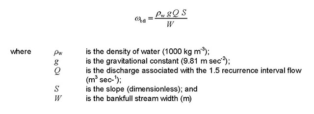
ωbfl = (ρwgQS) ÷ W
Where
- ρw is the density of water (1000 kg m-3);
- g is the gravitational constant (9.81 m sec-2);
- Q is the discharge associated with the 1.5 recurrence interval flow (m3sec-1);
- S is the slope (dimensionless); and
- W is the bankfull stream width (metres)
If the site to be altered has a natural flow regime, field measurements of suspended sediment, and channel form and habitat indicators at the site can be correlated with similar measurements at potential reference sites, as identified above, to build greater confidence in establishing a reference condition.
| Form and Transport Function | Bed Texture | Planform and sediment texture | Form, activity level and storage potential |
|---|---|---|---|
| Source Colluvial S>0.2 | Sand- bed S < 0.001 | 1. Braided Gravel Bed - only | Type 1 < 15 W/m2- Inactive |
| Transport Cascade 0.3>S>0.1 | Sand-Gravel 0.001 < S < 0.005 | 2. Braided Gravel Bed/Braided Sand Bed | Type 2 15-30 W/m2- Meandering |
Response (Kondolf et al. 2003) | Gravel/Cobble -bed 0.0005 < S < 0.005 Boulder-bed 0.005 < S < 0.05 Steep pool/fall S > 0.05 (Bathurst 1997) | 3. Wandering Gravel/Braided Sand 4. Low sinuosity and Meandering Sand Bend 5. Meandering Sand Bed only (Montgomery and Buffington 1999) | Type 3 30-60 W/m2 – Actively Meandering Type 4 60-100 W/m2 Type 5 100-200 W/m2 – Very Active – Braiding possible Type 6 > 200 W/m2 – Very Active – Large channels, finer grained, low sinuosity. W/d ratio decreases with increasing unit stream power. (Brooks 1988; Kondolf et al. 2003; Luce 2009) |
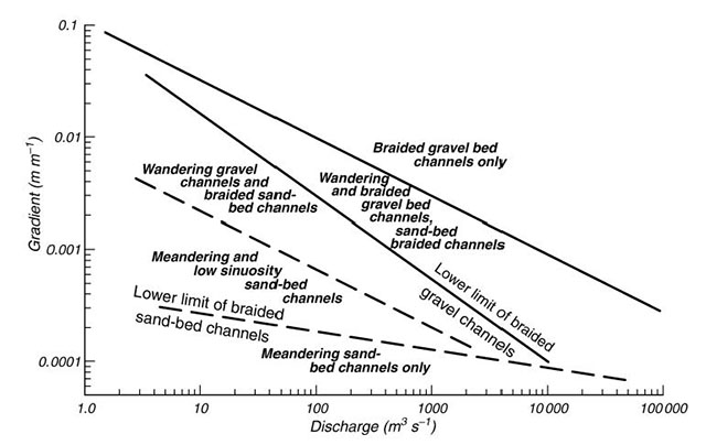
5.0 Information requirements
Information required to assess an alteration in the sediment regime and associated data sources are shown in Table 3.
| Information requirement | Data source |
|---|---|
| Assessment criteria values for the reference condition | Existing sediment and morphological records, aerial photos and remotely sensed imagery for the site (if natural) or for a reference site. |
| Indicator values for the current condition (if already altered) | Existing sediment and morphological records, aerial photos and remotely sensed imagery and field measurements. |
| Indicator values for the proposed post-alteration condition. | Information on the proposed design and operation of the facility as it pertains to the passage of sediment. |
Sediment regime indicators are assessed within defined field survey reaches that are located using the following criteria,
- Downstream of the proposed development: For the entire length of the downstream zone of influence, measure the river slope (S) using a Digital Elevation Model (DEM) or Ontario Base Map (OBM) at 1 channel width intervals and at breaks at slope to produce a long profile of the downstream ZOI. Use the breaks in slope to segment the river and classify the channel type of each segment using criteria presented in Table 2 and similarity of appearance in planform as viewed from aerial data such as Google Earth. If only one channel type exists in the downstream ZOI, locate the field survey reach at the second sampling site (see Chapter 1). If more than one channel type is identified, locate one field survey reach in each of the lengths of river between sampling sites 1 and 5 and 6 and 10 (or the last sampling site if less than 10) (see Chapter 1). Locate field survey reaches downstream of rapid changes in bed slope and/or in the most abundant channel type in each length of river.
- Upstream of the proposed development: Upstream of the reservoir (existing or proposed) select a reach that is geomorphically similar to a field survey reach downstream of the development. If deposition in the channel upstream of the development is a concern, select a field survey reach so the last cross section, at a minimum, will be located within the backwater effect of the proposed reservoir. Otherwise, ensure the field survey reach is upstream of this influence if it is to be used as a post-alteration reference site. If there is no reach upstream of the development that is comparable to a survey reach downstream of the reservoir, select a reach that is broadly representative of the channel form.
- Reference site: Select reaches with similar channel types as the development sites, weighting the stream power based classification and apparent geomorphic similarity heavily in the decision. If the upstream and downstream reaches at the development site are distinctly different, then try to select a reference site at an alternative location and select one with the same downstream transition in channel morphology. For example if the reach in the downstream ZOI transitions from a Type II to a Type III channel, look for a reference reach with the same type of downstream transition.
At each field survey reach, identify appropriate cross sections to meet the following criteria:
- Five (5) cross sections located at successive riffle-pool sequences (e.g. Riffle 1, Pool 1, Riffle 2, Pool 2, Riffle 3 etc.). Then, immediately downstream of the last cross section in this sequence, a series of another 5 cross sections located at 1 bankfull channel width intervals. These transects are to capture changes in the smaller scale river morphology not captured by the other 5 cross sections.
- All cross sections should be oriented perpendicular to the bankfull channel banks with a 3′ rebar stake monumented (i.e. the benchmark) at each end of the cross section. Locate the stakes ½ channel width from banktop to minimize the hazard of them being eroded away within a 20 year period.
- Riffle cross sections should be located 1/3 channel width upstream of riffle crest. The riffle crest is simply the highest point in the bed of the river between the two “pools”. Riffles and pools are not always apparent in some river types. Here, riffles and pools are defined in terms of the datum of the average bed elevation. If a point is higher than the average bed elevation, when considering a length of river 12-24 channel widths in length, then it is a riffle. The crest of which is the highest point. If the location is below the average streambed elevation then it is a pool. Thus, the definition of riffle and pool in this case is not based on hydraulic condition which varies with stage and stream type. The average bed elevation is most objectively determined using a regression of the long profile elevations. In practice in the field, the riffle crest can be observed on gravel bed simply by walking along the bed and noting the high point. In sand bed rivers, there is typically a flow convergence (V-shaped pattern on the water surface) at these high points in the bed. In deep river cases, a sonar unit can be used along the fastest zone of flow in the downstream direction to locate the points of higher than average bed elevation.
- Pool cross sections should be located at the deepest section of the pool or 1 channel width downstream of the bend apex.
To support the calculation of indicators and assessment criteria discussed below, the following should be measured at each cross section and the date and time of the measurements recorded to enable the measurements to be related to gauge records.
- The cross-sectional profile, measured between the rebar stakes using a graduated Kevlar tagline drawn taught for repeatable measurements. Divide the banktop width into 20 and measure bed elevations at each point. At the banks and at breaks in slope, survey points at ½ the increment. From the banktop to the rebar stake, survey points at 2× the increment to characterise the floodplain. This protocol will enable the most objective measure of bankfull characteristics and enable morphological change to be assessed.
- The waters edge elevation at each bank;
- Channel width at the bankfull flow;
- Channel depth at the bankfull flow;
- The long profile, measured from one channel width upstream of the first cross section, downstream to one channel width below the last (i.e. 10th cross section). Points should be taken at 1 channel width interval and at breaks in slope. The stadia rod should be placed in the deepest part of the channel along the thalweg, and at the waters edge. Also record the straight line distance;
- Grain size distribution classified using the Wentworth Scale (clay and silt [<0.0625 mm], sand [0.0625-2mm], small gravel [2-32 mm], large gravel [32-64 mm], cobble [64-256 mm] and boulder [>256 mm] and determined using methods such as:
- Wolman (1954) Pebble Counts across each cross section.
- Bulk sample on one point bar in the middle of the reach. The sample should be taken from the coarser, upstream 1/3 of point bar surface for surface sediments and (once surface sediments removed to depth of largest apparent mobile grain size) subsurface sediments. For sand bed rivers, the samples are small enough to be bagged and transported to the lab for sieve analysis. For deep sand bed rivers, a grab sampler will be required. For gravel bed rivers, on a tarp placed on the bar, divide the sample in two by running it through a coarse sieve (e.g. 32 mm) sieve. Record the mass of the coarse material pile and fine material pile. Take a 3-4 kg sub sample of the fine material for lab analysis. Pass the remaining coarse material through a set of coarse sieves and weigh the mass remaining on each sieve. Alternatively, a Wolman Pebble Count can be performed on the surface before sediments are removed and segregated.
6.0 Sediment regime characteristics, indicators, and assessment criteria
Methods to assess change in the sediment regime are provided below. In some cases, indicators and assessment criteria will be calculated using preliminary assessments, primarily desk-top methods, and refined, or in some cases replaced, with field-based assessments when such data can be collected.
6.1. Sediment transport – Suspended load
6.1.1. Description and rationale
Sediment supply is the availability of materials in drainage basins. Drainage basin geology and geomorphology are considered primary controls on the volume and size distribution of sediment supply and longitudinal pattern of sediment input (Stillwater Sciences 2006). Suspended sediment is the fine-grained load distributed throughout the water column. It is comprised of sediment delivered to the river from upland sources and that is sufficiently fine to remain in suspension at a given flow velocity (Hicks and Gomez 2003). Suspended sediment concentrations are generally considered to be limited more by the supply of fine sediment to the channel, rather than the capacity of flows to support it in suspension (Hicks and Gomez 2003). Continuity of downstream suspended sediment transport that supports the biologic and ecologic functioning of the channel is disrupted by in-stream structures by separating the upstream supply of sediment from downstream reaches and diminishing the capacity of flows to hold sediment in suspension.
The degree to which suspended sediment transport is interrupted is correlated to the trap efficiency of the impoundment created by an in-stream structure such as a dam. Trapping efficiency represents the percentage of suspended sediment delivered to the reservoir from the drainage basin, that will be trapped and settle out within the reservoir. It provides an indication of the degree to which the dam and headpond alters the conveyance of sediment from upstream to downstream river reaches, within the zone of influence. The trap efficiency of headponds and reservoirs is most often reported to be between 70 to 99% of the incoming sediment (Sundborg 1992; Toniolo and Schultz 2005; Wildi et al. 2010.) Most large dams are considered to trap virtually all of the sediment delivered from upstream (Petts 1984; Williams and Wolman 1984). Trap efficiencies for small dams vary more widely, ranging between 10 and 90% (Brune 1953; Meade et al. 1990; Grant et al. 2003; Huggett 2007).
6.1.2 Indicators
Mean annual suspended sediment yield
The mean annual suspended sediment yield indicator is the total weight of suspended sediment passing through a specific river cross-section, per unit area (i.e. upstream basin area), per year (tonnes/km2/year) averaged over the period of record. It is estimated differently in preliminary and field-based assessments owing to the differences in source data available at the two stages. In preliminary assessment, a surrogate may be used to estimate mean annual suspended sediment yield while field-based assessment builds on this initial desktop assessment by using field data.
Sediment yields are expected to be similar for similar sized drainage basins within an area of relatively uniform geology, physiography, climate, vegetation cover and land use, except under conditions when large discrete sediment sources are present (Reid and Dunne 2003). Church et al. (1999) have suggested that the dominance of lakes and predominately discontinuous glacial soils over hard rock like that found on the Canadian Shield, translates into very low sediment yields, exhibiting very little scale dependence. However, documented spatial anomalies in surficial geology can occur in this physiographic region and have significant impacts on sediment yields (Stone and Saunderson 1996).
The mean annual suspended sediment yield will be the most difficult of the sediment regime indicators to estimate because of the lack of data. Thus, all sources of available information should be used to estimate this indicator, assess the magnitude of change expected with the alteration, and predict possible biophysical consequences of the change.
6.1.3 Information requirements
6.1.3.1 Preliminary assessment
Calculation of the indicator requires either observed or interpolated suspended sediment data to establish the reference condition. Recommended methods for identifying suitable reference condition locations are included in Section 4.
6.1.3.2 Field-based assessment
Monthly suspended sediment samples of high flow and low flow events (i.e. 3 samples each = 6 samples) during open water conditions should be collected at a proposed development site for a minimum of one year to capture ‘average’ suspended sediment transport. All samples should be collected using suitable standard depth-integrated sampling methods (Edwards and Glysson 1999; Nolan et al. 2005). A minimum of three (3) samples should also be obtained during higher magnitude event flows, including spring and fall freshets, to provide a more thorough sample of these high suspended sediment load events.
These data will be used to validate and refine preliminary assessment estimates of suspended sediment yield. If the reference condition was established by transferring historical data from nearby monitoring sites, concurrent measurements from the development site and reference site are recommended to correlate the data and refine the estimates.
Suspended sediment measurements should be taken on the upstream cross section of the field survey reach.
6.1.4 Assessment criteria
If sufficient annual suspended sediment data is available, assessment criteria should include the annual sediment yields associated with the 13th, 38th, 62nd, and 87thpercentiles calculated using the reference condition mean annual suspended sediment yield data.
Otherwise, if the mean annual suspended sediment yield was estimated, the assessment criteria for the suspended sediment indicator would include the values (t/km2/year) associated with the standard errors (%) shown in Table 3 for rivers of similar size in the same Great Lakes Basin.
6.1.5 Evaluating alteration
When values for assessment criteria are derived from historical mean annual suspended sediment yield data from monitoring sites, the degree of alteration is evaluated as:
| Lake | Basin area (km2) | Number of basins | Mean annual suspended sediment load (t year-1) | Standarderror of mean (%) | Silt-clay load (%) | Mean annual sediment yield (t km-2year-1) | Standard error of mean (%) |
|---|---|---|---|---|---|---|---|
| Erie | 0-100 | 3 | 2 412 | 8.6 | 78 | 76 | 9.3 |
| Erie | 100-1000 | 9 | 29 916 | 7.5 | 78 | 76 | 6.9 |
| Erie | 1000-10 000 | 1 | 114 308 | 10.9 | 80 | 22 | 10.9 |
| Erie | > 10 000 | 0 | |||||
| Ontario | 0-100 | 14 | 4540 | 8.2 | 72 | 62 | 7.4 |
| Ontario | 100-1000 | 18 | 16 904 | 7.8 | 89 | 52 | 6.7 |
| Ontario | 1000-10 000 | 1 | 3885 | 15.4 | 100 | 2 | 16 |
| Ontario | > 10 000 | 1 | 39 062 | 22.6 | 100 | 3 | 22 |
| St Clair | 0-100 | 0 | |||||
| St Clair | 100-1000 | 3 | 24 319 | 8.7 | 96 | 100 | 9.6 |
| St Clair | 1000-10 000 | 2 | 205 911 | 11.9 | 94 | 68 | 5.4 |
| St Clair | > 10 000 | 0 | |||||
| Huron | 0-100 | 2 | 11 600 | 5.8 | 99 | 28 | 6.4 |
| Huron | 100-1000 | 12 | 22 899 | 12.5 | 99 | 38 | 8.9 |
| Huron | 1000-10 000 | 9 | 22 754 | 13.7 | 100 | 20 | 6.9 |
| Huron | > 10 000 | 1 | 1 357 434 | 8.8 | 100 | 98 | 8.8 |
| Superior | 0-100 | 2 | 37 523 | 11.2 | 100 | 23 | 8.9 |
| Superior | 100-1000 | 5 | 2958 | 10.2 | 97 | 5 | 11.5 |
| Superior | 1000-10 000 | 9 | 61780 | 16.3 | 84 | 31 | 7.8 |
| Superior | > 10 000 | 0 |
- Low alteration: A mean annual suspended sediment yield (t/km2/year) that lies between the 38thand the 62nd percentiles of the mean annual suspended sediment yield for the reference condition.
- Medium alteration: A mean annual suspended sediment yield (t/km2/year) that lies between the 13thand 38thor 62nd and 87thpercentiles of the mean annual suspended sediment yield for the reference condition.
- High alteration: A mean annual suspended sediment yield (t/km2/year) that is less than the 13thor greater than the 87thpercentile of the mean annual suspended sediment yield for the reference condition.
Where assessment criteria were based on the work of Stone and Saunderson (1996) the degree of alteration can be evaluated as follows:
- Low alteration: A mean annual suspended sediment yield (t/km2/year) that lies within the % associated with ± 1 standard error of the mean annual suspended sediment yield for the reference condition.
- Medium alteration: A mean annual suspended sediment yield (t/km2/year) that lies within the % associated with ± 2 standard errors of the mean annual suspended sediment yield for the reference condition.
- High alteration: A mean annual suspended sediment yield (t/km2/year) that lies beyond the % associated with ± 2 standard errors of the mean annual suspended sediment yield for the reference condition.
6.1.6 Methods
An extensive archive of suspended sediment data exist for select Water Survey of Canada, hydat stations in Ontario. These data are presented in various forms, including instantaneous suspended sediment, suspended sediment concentration and suspended sediment load, each collected using depth integrated samplers. Less frequently, the particle size distribution of bed materials may also be reported. Methods for identifying suitable sediment records in HYDAT to transfer to the development site are discussed in Section 4.
Online resources can be used to determine the location and suitability of sediment records using the following steps:
- Using the WSC hydrometric data Advanced Location Search (http://www.wsc.ec.gc.ca/applications/H2O/index-eng.cfm?stype=location)[link inactive] query the database to find stations in Ontario, with a ‘regulation type’ of natural, reporting sediment data, with a gross drainage area greater than 100 km2. A list of gauges meeting these query requirements will be generated.
- From the site list compiled in (a), develop a short-list of HYDAT stations located in the vicinity of the development site, by referring to the WSC Google Map tool (http://www.wateroffice.ec.gc.ca/google_map/google_map_e.html?search_by=p&province=ON) [link inactive]for active sites and other suitable spatial database for discontinued sites.
- Compare relevant basin attributes of the short-listed gauges from (ii) to those of the development site (see Section 4).
- Once a suitable reference drainage basin is identified, sediment data can be downloaded from the Water Survey of Canada’s Archived Sediment Data page (http://www.wsc.ec.gc.ca/sedat/sedflo/index_e.cfm?cname=main_e.cfm [link inactive]) by entering the site information (site name or HYDAT number) for the chosen site.
Suspended sediment data may be sparse because of infrequent sampling intervals at some HYDAT sediment stations. If sampling was conducted during high flow events, known to transport high concentrations of suspended sediments, the data could be biased upwards. For this reason, estimates of suspended sediment loads must be used to account for river discharge at the time of sampling. Clarke (1990) suggests that when instantaneous discharge data coinciding with the time of suspended sediment sampling are unavailable, daily discharge can serve as an appropriate surrogate. When load data are not included in the HYDAT sediment database, sediment concentrations can be combined with daily discharge to derive a measure of load (Clarke 1990). Further methods for suspended sediment load calculations and bias correction can be found in Porterfield (1972), Dickinson (1981), and Walling and Webb (1981).
Suspended sediment sampling should use the appropriate depth integrating suspended sampling apparatus and be consistent with standard suspended sediment sampling protocols (Edwards and Glysson 1999; Nolan et al. 2005).
Where sediment records do not exist, or are insufficient, approaches that relate basin characteristics to sediment conditions may be used (Summer and Walling 2002; Jinfa and Xiuhua 2004). Knowledge of potential sources of sediment supply within a river basin can also provide an initial indication of a river’s sediment regime (e.g. bedrock, glaciofluvial or lacustrine dominated substrates) as well as the relative importance of any sediment supply that might be directly affected by the development footprint (e.g. reservoir inundation).
Knowledge of the residence time and trapping efficiency (%) of a reservoir can provide an indication of the potential degree of alteration expected in the suspended sediment yield. Trapping efficiency of a reservoir can be calculated using the residence time:
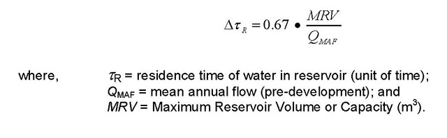
ΔτR = 0.67•(MRV ÷ QMAF)
where,
- τR = residence time of water in reservoir (unit of time);
- QMAF = mean annual flow (pre-development);
- MRV = Maximum Reservoir Volume or Capacity (m3).
Trapping efficiency (TE) of a reservoir is calculated using:
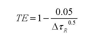
TE = 1 - [0.05 ÷ (ΔτR0.5)]
Values obtained represent % reduction in total sediment load.
6.2. Sediment transport - Bedload
6.2.1 Description and rationale
The habitat conditions of a river or stream are strongly associated with the river bed- material. The coarser sediments transported along the river bed also control the morphology of the channel and maintain the heterogeneity of aquatic habitat that is required by aquatic organisms during different stages of their lifecycles (Gordon et al. 2004). Because species differ in their substrate preferences and requirements, they depend on a mixture of particle sizes and interstices, among other attributes, to support colonization (Gordon et al. 2004). In this way, species have evolved along-side the dynamic equilibrium of the bedload sediment regime. However, the continuity of downstream bed-material transport that supports the biological and ecological functioning of the channel is disrupted by instream development such as dams, which alter the sediment supply and flow competencies to support bedload transport (Curtis et al. 2010).
Bedload transport is commonly thought of as a two-phase process. Phase I transport consists of sand and small gravel moving at relatively low rates over a stable channel surface. Phase II transport rates are considerably greater as gravels and larger sized material are moved, including material from both the channel surface and subsurface (Ryan et al. 2002). The initiation of Phase II transport defines the starting point of significant bed mobility and channel change if the upstream sediment supply changes, (Schmidt and Potyondy 2004). Schmidt and Potyondy (2004) refer to this threshold of Phase II transport in terms of a critical discharge (Qtrigger). This critical discharge is synonymous with the “channel maintenance flow”.
Estimation of bedload transport rates and loads in the field is challenging. In wadeable rivers, field based methods include the use of either hand held bedload samplers or trapping devices that are left on the streambed during floods (e.g. Bunte et al. 2007). On larger rivers, bedload samplers are deployed from a boat or bridge that spans the river (see Edwards and Glysson 1999). If bedload measurements are not feasible, estimates of bedload transport rates can be calculated from properties of flow and bedload transport equations. In practice, this modeling approach is commonly used given the difficulties of making direct measurements (Wilcock 2004). Bedload transport equations typically relate a property of flow (e.g. discharge Q, shear stress t, stream power ω) to the transport rate. Sediment transport is initiated when the magnitude of the flow property exceeds a critical threshold (e.g. Qcrt, tcrt, wcrt). For convenience, discharge is often used in screening level assessments for bedload predictions, despite the fact that models predicting bedload transport based on discharge are often inaccurate (Gomez and Church 1989) due to the difficulty of determining an appropriate value for Qcrt. When field data are lacking, one can use a characteristic discharge, for example the bankfull discharge, as a discharge threshold to evaluate how changes in flow might affect channel form. Bankfull discharge has often been equated with channel-forming or effective discharge (i.e. the flow that does the most geomorphic “work”). Bankfull discharge (see Chapter 2 Section 6.4) has traditionally been considered to have a recurrence interval of approximately 1.5 years (Leopold et al. 1964), thus channel- forming flows can be generally expected to occur two out of every three years, occurring mostly during the spring “flood” flows.
More rigorous assessments of bedload transport rates typically employ the use of bed shear stress or stream power. Fractional transport equations can be used to calculate how changes in the flow properties affect selected target bed sediment sizes of ecological importance or ambient grainsize distributions as measured in the field (Schmidt and Potyondy 2004; Ryan et al. 2005). These approaches focus on the conditions necessary to entrain bed particles.
6.2.2 Indicators
Indicators for bedload transport are related to the critical discharge (Qcrt) and thus, are strongly linked to the hydrologic regime presented in Chapter 2. While the preliminary assessment indictor uses a variant of the Bankull Flow indicator referred to in Chapter 2 to estimate Qcrt, a more detailed assessment of bed load movement using field data is used in the field-based assessment. In this case of equating Qcrt to the critical discharge using bankfull flow conditions, Qcrt is not a threshold for the initiation of sediment movement but a threshold for the channel maintaining transport conditions. That is, the bed may be mobile before bankfull conditions but the transport that occurs at bankfull is the right combination of frequency and magnitude to do the most work in terms of channel maintenance. In other cases, Qcrt can be calculated for certain grain size fractions of interest. In this case, Qcrt does refer to the discharge at which these grains are entrained by flow.
6.2.2.1 Preliminary assessment
Annual bankfull flow duration
Annual bankfull flow duration is the percent time per year that the bankfull flow magnitude is equaled or exceeded. This builds on the Bankfull Flow indicator used in Chapter 2 but focuses specifically on the geomorphological aspects of these high flows. Of interest here is simply the amount of time that a river is maintaining transport conditions and how that duration might change with a planned alteration to the flow regime.
6.2.2.2 Field-based assessment
Annual excess stream power
Stream power is the time rate at which work is done or energy is expended and is a useful measure of a river’s erosive capacity (Gordon et al. 2004). Unit stream power is the total stream power standardized by the width of flow. The unit stream power provides an estimate of the mean value of stream power per unit of river bed area (Ferguson 2005) and is given by:
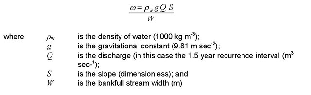
ω = (ρwgQS) ÷ W
where
- ρw is the density of water (1000 kg m-3);
- g is the gravitational constant (9.81 m sec-2);
- Q is the discharge (in this case the 1.5 year recurrence interval (m3sec-1);
- S is the slope (dimensionless); and
- W is the bankfull stream width (m)
In Section 4, we used the bankfull channel width because we were interested in the bankfull stream power. In channels with relatively vertical banks, the bankfull width can also be assumed as the width to be used in the calculation of stream power over a range of discharge conditions.
The critical stream power (ωcrt) defines the magnitude of energy expenditure required before channel bed material of a given size (Dx) will move and is controlled by the near- bed velocity of water moving downstream. Estimates of critical stream power for certain indicator bed material sizes are important for prescribing certain flow magnitudes to maintain the bedload transport regime or evaluate certain conditions that scour biota from the streambed. The critical stream power equation for motion for a given bed sediment size (Ferguson 2005) is used to calculate discharges to initiate bed sediment transport (See Section 6.2.6).
The threshold of incipient bedload motion occurs when:

ω = ωcrt
The bedload transport rate increases exponentially as a function of the excess stream power above the critical threshold:
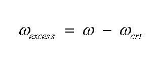
ωexcess = ω - ωcrt
Thus, the sum of excess stream power calculated from a flow series is proportional to the total load that was transported.
If the mean unit stream power is greater than the critical stream power (ω > ωcrt), particles are being mobilized from their rest position on the bed and transported downstream. If the reach is in equilibrium in terms of sediment supply, where the amount of sediment supplied from upstream is equal to the amount being transported downstream, then no morphological change results. If the duration and magnitude of transport increases for that site, but the sediment supply of that grain size fraction does not change, then the channel boundary will erode (i.e. the grain size fraction will persist on the bed). Alternatively, if the duration and magnitude of transport decreases for a given sediment supply, then deposition of that grain-size fraction is likely to increase (aggradation). When the bankfull stream power is considered in this type of analysis, it is intended to be representative of the transport of a whole range of grain size fractions and thus, gives an indication of the likelihood of reach-scale aggradation or degradation (not just individual grain size fractions).
Similarly, transport calculations are often based on the median grain size of a sediment distribution (D50) under the assumption that when the average grain size is in motion, all of the grain sizes are mobile. However, researchers have demonstrated that the amount of fine sediment on the bed makes the bed more susceptible to transport (Wilcock and Kenworthy 2002). To capture the initiation of bedload erosion from the river bed (which is the onset of channel change), Ryan et al. (2005) indicated that the movement of the D16 to D25 grain sizes seemed to correspond with the onset of Phase II transport (discussed earlier); thus, these grains sizes are used for the field-based assessment indicators rather than the D50.
6.2.3 Information requirements
6.2.3.1 Preliminary assessment
Calculation of the bedload erosion indicator requires a streamflow time series (natural flow simulation i.e. reference condition, or observed) at the site of the flow alteration. Recommended methods for establishing the reference condition are provided in Chapter 2, Appendix I, Section 1.1.
6.2.3.2 Field-based assessment
In the field-based assessment, field measurements of channel characteristics at each field survey reach are used. The channel form and substrate should be characterized using the cross-channel transect approach discussed in Section 5. This includes undertaking Wolman (1954) Pebble Counts and obtaining bulk substrate samples to estimate bed sediment size distribution and characteristic grain size fractions (e.g. 2 mm sand, D16, D25, D50 ). The Di notation refers to the frequency distribution of sediments sampled, where D50 equals the particle size that 50% of the sample bed sediments are equal to or smaller than. The D25 is the particle size that 25% of the sampled bed sediments are equal to or small than, etc. Bed sediment analyses should characterise these grain sizes (D16, D25, D50).
If the natural flow simulation used in preliminary assessment has been refined through field-based assessment, the latter should be used to improve the stream power estimates.
6.2.4 Assessment criteria
6.2.4.1 Preliminary assessment
Assessment criteria for the annual excess stream power indicator include the values associated with the 13th, 38th, 62nd, and 87thpercentiles expressed as the percent time (duration) the critical stream power values associated with the D16, D25, D50, grain sizes are equaled or exceeded annually.
6.2.5 Evaluating alteration
6.2.5.1 Preliminary assessment
Alterations in preliminary assessment indicators are evaluated as follows:
Low alteration: The annual bankfull flow duration (%) lies between the 38thand the 62nd percentiles of the annual bankfull duration for the reference condition.
Medium alteration: The annual bankfull flow duration (%) lies between the 13thand 38thor 62nd and 87thpercentiles of the annual bankfull duration for the reference condition.
High alteration: The annual bankfull flow duration (%) is less than the 13thor greater than the 87thpercentile of the annual bankfull duration for the reference condition.
6.2.5.2 Field-based assessment
Alteration in field-based assessment indicators are evaluated as follows:
Low alteration: The annual excess unit stream power duration for 2mm Sand, D16, D25, and D50 grain size materials lies between the 38thand the 62nd percentiles of the annual unit stream power duration for the reference condition.
Medium alteration: The annual excess unit stream power duration for 2mm Sand, D16, D25, and D50 grain size materials lies between the 13th and 38th or 62nd and 87th percentiles of the annual unit stream power duration for the reference condition.
High alteration: The annual excess unit stream power duration for 2mm Sand, D16, D25, and D50 grain size materials is less than the 13th or greater than the 87thpercentile the annual excess unit stream power duration for the reference condition.
6.2.6 Methods
For each cross section in the field survey reach (Section 5), estimate the critical stream power for incipient motion for a given grain-size fraction of interest (ωcrt W m-2) (Ferguson 2005).
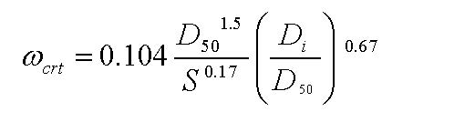
ωcrt = 0.104 × (D501.5/S0.17)(Di/D50)0.67
Where
- D50 is the median grain size (metres);
- Di is the given grain-size fraction of interest (metres); and
- S is the water surface slope.
We can then rearrange the unit stream power equation to calculate the discharge (Qcrt) associated with the critical stream power (ωcrt),
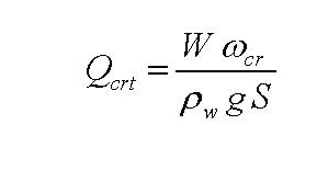
Qcrt = (Wωcr)/(ρwgS)
We can then calculate the duration of time when
Q > Qcrt
by using the flow duration curve of the associated streamflow time series.
6.3 Channel form and habitat
6.3.1. Description and rationale
Fluvial geomorphology not only includes processes related to the erosion, transport, and deposition of sediment but also the channel form that results from these processes. Channel form can be described in three dimensions: by its pattern (planform), slope (longitudinal profile) and cross-section (transverse section) (Petts and Foster 1985). Measures of these characteristics provide further information about the interactions of flow, parent material, and the sediment regime. A river’s channel form ultimately controls the amount and heterogeneity of biotopes important for maintaining the ecological condition of a river and specific habitat requirements of VECs.
6.3.2 Indicators
Sinuosity Index (SI)
Channel pattern is the term used to describe the planform view of a river reach or entire river as seen from a ‘birds-eye’ view. This channel pattern reflects the hydrodynamics of flow within the channel and associated processes of energy dissipation and sediment transfer (Eziashi 1999). The sinuosity of a stream is related to hydraulic and topographic factors and can be measured using the sinuosity index (SI) (Mueller 1968) which is the difference between channel length and valley length. Sinuosity has been used to discern the downstream impacts of in-stream structures such as dams as an analog for channel stability (Martson et al. 2005). Positive relationships between sinuosity index and in- stream habitat have been identified, where rivers with higher sinuosity indices are considered to support a more diverse aquatic community compared to river sections with a lower sinuosity index (Fukushimi 2001; Lohani 2008). Others have identified a higher habitat heterogeneity per unit distance in rivers with a high SI index (Goldstein et al. 2002; Ohio EPA 2010). Thus, alterations on rivers with higher SI values will be associated with higher degree of change to ecological condition and VEC state compared to rivers with lower SI values.
6.3.3 Information requirements
Calculation of a sinuosity index requires up-to-date planform maps or higher resolution imagery, including aerial photography or remotely sensed imagery, of the river channel focusing on the downstream zone of influence.
6.3.4 Assessment criteria
Assessment criteria for the sinuosity index are based on some commonly used classes of SI for single channel rivers. These, include: a) straight (SI < 1.05); sinuous (SI 1.05- 1.5), and: meandering (SI > 1.5) (Mount 1995; Gordon et al. 2004).
6.3.5 Evaluating alteration
The potential change to ecological condition and VEC state increases as the sinuosity decreases, associated with the straightening of a channel.
Low alteration: The sinuosity index remains in the SI class associated with its reference condition.
Medium alteration: The sinuosity index is one SI class removed from the reference condition.
High alteration: The sinuosity index is two SI classes removed from the reference condition.
6.3.6 Methods
The sinuosity index for the downstream zone of influence is determined by the ratio of channel length to downvalley length given by the equation (Knighton 1998) (Figure 2):
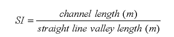
SI = channel length(metres)/straight line valley length (metres)
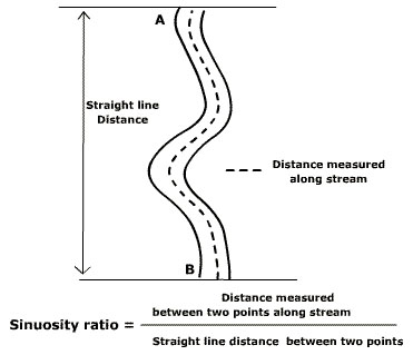
6.3.7 Indicators
Mean width-depth ratio
Width-depth ratio is an indicator of channel shape and is used for assessments of changing discharge and sediment load on channel morphology (Chorley et al. 1984). Resurveying established cross-sections along reaches of a river in locations that might be susceptible to erosion and/or sedimentation is one of the most straightforward methods to measure physical change in rivers. Generally, width-depth ratios increase with increasing stream power and bank erodibility (Robertson-Rintoul and Richards 1993; Brandt 2000). The width-depth ratio is a key variable for assessing change in channel dynamics, particularly changes between sediment load and capacity. Increases in width-depth ratio generally are associated with accelerated streambank erosion, excess deposition/aggradation processes, over-widening due to direct mechanical impacts, and other causes. Examples of width-depth ratio responses to changes in sediment capacity, competency, and flow are shown in Figure 3.
6.3.8 Information requirements
Measurements of bankfull width and bankfull depth at each cross section of each field survey reach.
6.3.9 Assessment criteria
Assessment criteria for the width-depth ratio indicator include the values associated with one and two standard deviations from the mean width-depth ratio of the reference condition.
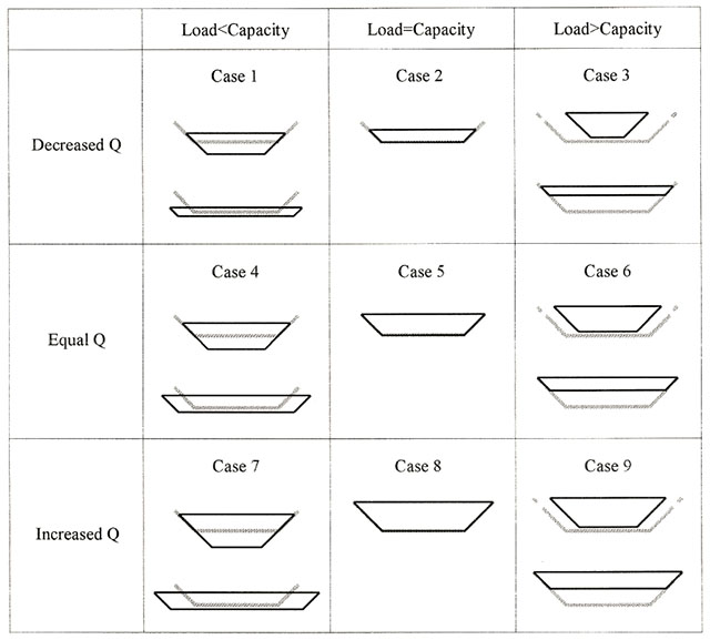
Some general observations on width-depth ratios include:
- W-D Ratio < 10
- small bedload and high suspended load
- typically channel is narrow and deep
- 10 > W-D Ratio
- intermediate bedload, intermediate bedload
- mixed load channel
- W-D Ratio < 40
- higher bedload
- lower suspended load
- lower sinuosity
6.3.10 Evaluating alteration
Low alteration: A mean width-depth ratio that is within values associated with one standard deviation of the reference condition.
Medium alteration: A mean width-depth ratio that is within values associated with two standard deviations of the reference condition.
High alteration: A mean width-depth ratio that is beyond values associated with two standard deviations of the reference condition.
6.3.11 Methods
The width-depth ratio is calculated by dividing the bankfull width by the mean bankfull depth. Methods for identifying bankfull stage in the field is provided in Section 2.2 of Chapter 2 Appendix I.
6.3.12 Indicators
Bed composition
Bed composition, including the size and distribution of particles is an indicator of in- stream channel change used to assess the effects of changing discharge and sediment load on channel bed and bank morphology (Chorley et al. 1984; Wilcock et al. 2009). The distribution and size of bed materials can change significantly following the construction of dams (Grant et al. 2003; Salant et al. 2006). The amount of geomorphic adjustment is generally dependent on dam operation, associated alteration to hydrologic regimes and the characteristic mode of sediment transport in a channel (Brandt 2000; Schmidt et al. 2001; Dade et al. 2011). Alterations to the natural dynamic equilibrium of sediment erosion and aggradation can lead to impacts on bed related habitat (Kondolf et al. 2008). For instance, where dams eliminate supplies of smaller mobile gravels, bed material may become too coarse for spawning fish to move (Parfitt and Buer 1980) and excessive levels of fine sediment can clog spawning gravels (Sear et al. 2008). In cases where increased sedimentation occurs downstream of dams, embeddedness (the degree to which fine sediments surround coarse substrates on the stream bed) can increase (Sylte and Fischenich 2002; Sennatt et al. 2006). Increased embeddedness has been correlated with degraded benthic habitat and declines in macroinvertebrate abundance and diversity (Waters 1995; Angradi 1999).
The composition and nature of the river bed can be an early indicator of changes in sediment regime with concurrent impacts on invertebrate production, biomass, and fish production. Morphological changes in riffle shape and substrate composition may reduce their suitability for the reproduction of certain species of fish.
6.3.13 Information requirements
Information on bed composition is collected using the Wolman Pebble Count and bulk sample methods outlined in Section 5.
6.3.14 Assessment criteria
Alteration in bed composition is assessed, ideally, by examining change in the entire grain size distribution. Of particular interest for calculations in this chapter are changes in the values associated with the % composition for the D16, D25, and D50 grain sizes. In predicting potential shifts in bed composition in response to an alteration, the bed composition indicator focuses on the D50 grain size.
6.3.15 Evaluating criteria
Low alteration: The bed composition indicator lies between the 38thand the 62nd percentiles of the grain size distribution for the reference condition.
Medium alteration: The bed composition indicator lies between the 13thand 38thor 62nd and 87thpercentiles of the grain size distribution for the reference condition.
High alteration: The bed composition indicator is less than the 13thor greater than the 87thpercentile of the grain size distribution for the reference condition.
6.3.16 Methods
Characterization of river bed material is achieved using Wolman Pebble Counts and bulk samples as described in Section 5.
7.0 Supporting information
The following information is suggested to accompany a sediment regime assessment. This will allow an adequate evaluation of the quality of the information and analyses used to estimate values for indicators and assessment criteria and for the interpretation of results:
- A table comparing drainage basin area (km-2), landscape characteristics (surficial geology, mean slope and percent area covered by water) and the river-bed characteristics (e.g. percent underlying surficial geology) for the drainage basin upstream of the development site and for all sites assessed as potential reference sites.
- A table identifying HYDAT sediment stations used in sediment yield analysis, including a rationale for their use.
- A list of any non-natural (anthropomorphic) impacts upstream of the proposed site (e.g. river alteration, mining, forestry, industry etc.) that might be influencing sediment yield and the percent area of the upstream drainage basin they occupy.
- The anticipated maximum reservoir or headpond volume or capacity (m3) and residence time of water in reservoir.
- Diagrams of longitudinal profiles scaled appropriately in m m-1, noting any vertical exaggeration, for: i) the river extending from the upstream ZOI to the doswnsteam ZOI showing locations of the in-stream development and reservoir (existing or proposed) with all sampling site locations demarcated; and ii) the field survey reaches with all cross sectional survey locations demarcated. Geographic coordinates of start and end points for the profiles should also be provided.
- Detailed diagrams of all river channel cross section surveys, identifying channel morphology and heights through the cross section, intervals used, including identification of bankfull stage and width. Details of the bank morphology and pictures taken to describe the site. Geographic coordinates of start and end points of all cross sections examined should also be provided.
- The locations of sinuosity measurements, identified using imagery or by geographic coordinates.
- Tables and graphs showing the complete grain size distributions obtained from the one bulk sediment sample from each field survey reach and from the Wolman pebble counts at each cross-section
- A plan view map showing the location of the each field survey reach, cross sections, longitudinal profile, and locations of in-stream structures.
8.0 Post-alteration monitoring
Post-alteration monitoring of the sediment regime requires measurement of continuous discharge as described in Chapter 2 Section 7 and suspended sediment sampling to measure annual suspended sediment load upstream and downstream of the waterpower facility following the sampling strategy described in Section 6.1.3.2.
All measurements taken at the field survey reach cross sections or from planform maps or aerial imagery should be repeated using the sampling frequency outlined in Chapter 1. This will document any changes in the physical character of the river bed structure and composition.
Chapter 4: Water quality
1.0 Introduction
Water quality in riverine ecosystems is a function of a complex interaction between hydrologic, atmospheric/climatic (e.g. solar energy input), watershed (e.g. soils/geology, topography), and biotic variables. Chemical characteristics like dissolved oxygen (DO), alkalinity, pH, and nutrients, and physical characteristics like water temperature, turbidity and light transmission, are all influenced by flow regime, climate/weather, geology and land use patterns, and sources of organic matter. Together with the flow, sediment, and temperature regimes, these water quality properties strongly influence river productivity and biodiversity.
This chapter focuses on water quality factors that most strongly shape the ecological condition of river systems and that are often of greatest importance to the health of valued ecosystem components like species at risk or socio-economically important fish species. The purpose is to provide the information needed to assess potential changes to these indicators resulting from in-stream development. However, the principles and indicators described here can be used to help assess the effects of any type of project that will change riverine water levels or flows.
2.0 Rationale
Water quality strongly influences the structure and functioning of aquatic ecosystems. Alteration of water quality characteristics beyond the range of natural variability can cause changes in productivity (Clark et al. 2008; Wooton et al. 1996), shifts in biological communities that result in shortened food webs (Clark et al. 2008; Marty et al. 2008; Marks et al. 2000; Spence and Hynes 1971;) and reduced biodiversity (Bunn and Arthington 2002; Rosenberg et al. 1997; Coleman 1996).
The flow regime is the dominant variable affecting water quality in rivers and lakes (Sokal et al. 2009). Changes in flows and levels caused by in-stream developments can have significant effects on water quality, both upstream and downstream. For example, reductions in flow at a dam or within a reservoir increase the deposition of sediments (Petts 1984), alter nutrient transport and recycling processes (Vannote et al. 1980: Ward and Stanford 1989; Junk et al. 1989, Ittekkot and Haake 1990 in Rosenberg et al. 1997) and affect the downstream sediment regime (Knighton 1998; Bowen et al. 2003, Shields et al. 2000). The composition and concentrations of nutrients and suspended sediments in water strongly influence a river’s primary productivity and the types of biological communities it can support.
Reservoirs act as effective nutrient sinks, particularly for nutrients such as phosphorus (Friedl and Wüest 2002) and nitrogen (Marty et al. 2008). Increases in nutrient availability can stimulate primary production and lead to eutrophication, particularly in reservoirs where increased water residence times and higher water temperatures can create ideal conditions for phytoplankton and macrophyte growth. The additional organic matter resulting from higher primary productivity increases microbial decomposition and can lead to depletion of dissolved oxygen (DO) within the reservoir. Depending upon the design and operation of a dam, low DO water can be released downstream. Low DO concentrations can have a variety of lethal and sub-lethal effects on aquatic organisms (Doudoroff and Shumway 1970; Alabaster and Lloyd 1982) and increase the release of nutrients and contaminants like mercury from sediment (CCME 2003).
Suspended sediment levels determine turbidity and the depth of light penetration (Sokal et al. 2009) and hence, the amount of solar radiation available to algae and macrophytes (Krebs 1978; Rosenberg et al. 1997). Changes in light penetration can, in turn, affect fish behaviours such as predation, foraging efficiency, and nest protection.
A potential effect of large dams is the entrainment of high levels of atmospheric gases as water moves over a dam or through penstocks. Supersaturation of water with dissolved gases can lead to gas bubble trauma in fish and invertebrates. However, the severity of the effects varies among species (Clarke et al. 2008; Backman and Evans 2002; Backman et al. 2002) and must be assessed on a case by case (or species by species) basis.
Water temperature is a critically important characteristic that can be affected by in- stream development. Temperature directly influences the productivity of aquatic ecosystems through its effects on dissolved oxygen levels, carbon cycling and the ability of water to hold nutrients in solution (Poff et al. 1997; Olden and Naiman 2009). Temperature also plays a vital role in determining the presence or absence, life histories and spatial distribution of organisms in streams (Ebersole et al. 2001, Vannote et al. 1980). In particular, many critical life history processes in fish are regulated by temperature (Hauer and Hill 2007).
In summary, changes in flows and levels caused by in-stream developments can have significant effects on water quality and hence ecological condition both above and below a structure. Careful pre-alteration assessment and post-alteration monitoring can help to identify and evaluate potential effects of a development and options for mitigating them.
3.0 Indicator summary
| Characteristic | Indicator(s) |
|---|---|
| Dissolved Gases | Dissolved Oxygen Concentration |
| Dissolved Gases | Total Dissolved Gases* |
| pH | pH |
| Alkalinity | Alkalinity |
| Conductance | Specific Conductance |
| Dissolved Solids | Total Dissolved Solids |
| Suspended Solids | Total Suspended Solids |
| Light Transmission or | Secchi Disk Depth or |
| Turbidity | Nephelometric Turbidity |
| Nutrients Phosphorus | Total Phosphorus |
| Nitrogen | Nitrate/Nitrite |
| Nutrients Nitrogen | Total Ammonia |
| Nutrients Nitrogen | Total Kjeldahl Nitrogen |
| Organic Matter | Dissolved Organic Carbon |
| Primary Productivity | Chlorophyll-a concentration |
* Sampled only if facility design or operating plan are likely to cause increased oxygen entrainment.
Note: During the approvals process for water power projects, MOE administers the Permit to Take Water process, which also requires the collection of water quality data. As a result, the information needs for many of the indicators discussed here may be satisfied through their requirements.
4.0 Establishing a reference
To properly assess the potential effects of in-stream development on water quality and the ecological condition of a river, it is important to first understand the water quality regime of the site in its natural and current states. This information allows better estimates of the potential for changes in water quality resulting from an in-stream development, in order to answer the question “Is the planned project likely to cause changes in water quality that will affect aquatic ecosystem values?”
The purpose of the pre-alteration water quality assessment is to characterize current water quality conditions and provide a reference for estimating potential ecological changes associated with an in-stream development, establishing possible mitigation strategies, and identifying post-alteration monitoring requirements.
Data to establish a natural reference condition for water quality is typically more available than other types of data, since water quality is often measured by monitoring programs and as integral parts of many studies. However, when determining reference conditions, care must be taken to ensure that the data used are of high quality and that any differences in collection and analysis methods can be taken into account.
5.0 Information requirements
5.1. Preliminary assessment
The first step in assessing potential changes in water quality associated with an in- stream development is to determine if data are available to establish a reference and/or condition for the indicators of interest. Ideally, these would consist of multi-year time series from sampling locations above, below, and at the location of the proposed alteration. However, any available data for the site (or similar nearby sites) or a suitable model, may help inform the first stage of the assessment, the goal of which is to provide a rough indication of the potential effects of the alteration on the indicator of interest. For water quality indicators, existing data may be available from monitoring programs such as the Provincial Water Quality Monitoring Network (PWQMN)
If sufficient data or suitable models are available to make a preliminary assessment of the effects of the proposed alteration and this assessment suggests a low impact, then field sampling may be not be required. However, if sufficient data or models aren’t available to make an informed judgement, or if examination of the data or modeling results suggest the potential for significant ecological changes, then field sampling will be required. Field sampling should also be done if effects on sensitive ecosystem components (e.g. endangered species) or biodiversity are anticipated.
5.2. Field-based assessment
Field sampling will provide more detailed information of the water quality regime upon which to make an informed judgement about the effects of an in-stream development. Ideally, field sampling would be conducted for a minimum of 2 to 3 years prior to the alteration to increase the likelihood of capturing the range of variation representative of each indicator at that particular site. The shorter the time over which pre-construction data is collected, the more difficult it is to make scientifically defensible inferences about the current state of the river and how it may change because of the structure.
6.0 Measuring indicator variables – sampling design
Water quality indicators described in this chapter were chosen to represent key ecosystem components thought to be important determinants of ecological condition and the state of valued ecosystem components (VECs). Indicator selection was based on the scientific literature and advice provided through an MNR hosted workshop on indicators for effectiveness monitoring for water management planning (ESSA Technologies, 2005).
6.1. Selecting site-specific water quality indicators
Decisions about which indicators to measure and how to measure them should be based on site-specific characteristics, the type of alteration, and a priori knowledge of the potential for changes in the indicator variables. Sampling methods and the type of equipment used will vary. The general sampling guidelines below apply to all indicators, unless otherwise noted in the detailed indicator description.
Although each indicator is discussed separately, many of the variables can be measured simultaneously. For example, dissolved oxygen, conductivity, pH, and temperature are often measured at the same time using a hand-held probe. Similarly, a single water sample can often be analyzed for multiple nutrients. Sampling requirements should be developed with advice from the laboratory that will analyze the samples.
A general reference on water quality sampling methods is the Canadian Council of Ministers of the Environment document “Protocols Manual for Water Quality Sampling in Canada” (CCME, 2011). Up to date methods are also described in Standard Methods for the Examination of Water and Wastewater (Eaton et al. 2005, or online at Standard Methods website).
6.2. Selecting sampling sites
Sites for sampling water quality must be carefully selected to ensure they accurately characterise the condition for the indicator of interest. General guidelines for selecting sampling sites include:
- Sample at a minimum of 4 locations (see sampling sites identified in Chapter 1):
- In the upstream ZOI
- At sample sites 1, 5 and 10 (or the most downstream site) in the downstream ZOI.
- Additional sampling sites may be required in the bypassed natural channel reach if it contains ecologically important habitat, a valued ecosystem component, or if there is concern about maintaining its ecological integrity.
- Where pre-existing data are available, if feasible, use the same sampling sites to maintain continuity of long term records and take maximum advantage of the existing data.
- For new alterations at existing in-stream structures, sampling should continue at existing reference sites if already established.
Unless specified below for an individual indicator variable, three replicate samples should be acquired in the river’s thalweg. The three replicate samples may come from three depth integrated water samples or three in-situ probe measurements at each specified depth.
6.3. Selecting sampling depths
The greater the proportion of the water column integrated in the sample, the more useful the data are for making inferences about potential changes in the indicator being measured. If the river being sampled is deep or contains deep pools that provide important habitat for fish or other aquatic species, samples taken at multiple depths in the water column may be required to adequately characterize water quality.
With modern instrumentation, water column profiles (samples taken at regular depths throughout the water column) of many water quality characteristics described here can be taken quickly and easily. If this type of sampling is conducted, collection of water column depth profiles at 0.5 m to 1 m depth increments is recommended. If not feasible, samples from discrete depths can be collected using samplers designed for this purpose, such as Kemmerer or Van Dorn water samplers. Recommended depths for fixed-depth samples are 0.3 m - 0.5 m below the surface, mid-water, and 0.5 – 1.0 m from the bed. Modifications to these recommendations may be required depending upon the indicator, the depth of the river, and the amount of variability in water levels.
In small rivers and streams, water depths may be shallow enough to preclude taking samples at multiple depths. In these locations, water sampled at a single depth, usually 0.3 m – 0.5 m will usually provide a representative sample.
6.4. Determining sampling frequency
Water quality characteristics can vary on short times scales and often measurements during events such as transient high flow periods are the most important for assessing potential effects on ecological integrity. Modern instrumentation makes high frequency in situ monitoring of water quality variables possible, and in many cases more economical than sampling with bottles or hand-held instruments. Therefore, whenever feasible, the use of in situ samplers is recommended.
When in situ monitoring is not possible, and for variables that cannot be measured with in situ instruments, the sampling frequency must be carefully selected to ensure the representative seasonal and higher frequency variation in the indicator is captured. Indicator-specific sampling recommendations are included in the description of each water quality characteristic below. However, general best practices for determining sampling frequencies include:
- Sample more frequently when rates of change in the indicator are high and less frequently when they are low. For example, monthly sampling may be increased to weekly during high flow periods for some indicators (see individual characteristics).
- Sampling may be necessary across a range of flow conditions (low, medium, and high) in order to establish a relationship between the variables (e.g. turbidity and total suspended solids).
- If nutrient and sediment issues are anticipated, daily sampling may be necessary to capture transient events.
- Depending upon the system and the operating plan for the in-stream structure, lower frequency sampling may be sufficient for post-alteration monitoring of some indicators. However, for most variables, a minimum of 12 samples per year (monthly sampling) is recommended.
- Frequency of sampling should also consider potential rates of change for the indicator.
- For valued ecosystem components such as SAR, additional sampling may be desirable during critical times such as spawning periods.
| Indicator(s) | Sampling Frequency |
|---|---|
| Dissolved Oxygen Concentration | Monthly; weekly during low flow |
| Total Dissolved Gases | Monthly; targeted high flow periods |
| pH | Monthly; weekly during low flow |
| Alkalinity | Monthly; weekly during low flow |
| Specific Conductance | Monthly; weekly during low flow |
| Total Dissolved Solids | Monthly; weekly during low flow |
| Total Suspended Solids | Monthly; targeted daily during high/low flows |
| Secchi Disk Depth or Nephelometric Turbidity | Monthly; targeted daily during high/low flows |
| Total Phosphorus | Monthly; weekly during low flow |
| Nitrate/Nitrite | Monthly; weekly during low flow |
| Total Ammonia | Monthly; weekly during low flow |
| Total Kjeldahl Nitrogen | Monthly; weekly during low flow |
| Dissolved Organic Carbon | Monthly; weekly during low flow |
| Chlorophyll-a concentration | Weekly; Monthly for post-construction monitoring |
7.0 Assessment criteria
When assessing the potential effects of an in-stream development on ecological condition, the predicted post-alteration value of the indicator should be compared against the reference condition to determine the degree of alteration from both the reference (natural) condition and the current condition (if the river is not in its natural state). The mean and standard deviation of indicator variable values for the reference condition, or current condition, are used as assessment criteria unless otherwise stated in the indicator sections below.
8.0 Evaluating alteration
The degree of alteration for an indicator can be characterized as follows:
Low alteration
Estimated value of the indicator lies within one standard deviation of the reference condition.
Medium alteration
Estimated value of the indicator lies within two standard deviations of the reference condition.
High alteration
Estimated value of the indicator exceeds two standard deviations of the reference condition.
When the potential effect of a facility on a valued ecosystem component is of interest, the predicted post-alteration value of the indicator should be compared against known physiological requirements for the various life stages of the species of interest. The potential effect should then be qualitatively characterized as low, medium, or high based on the estimated impact to the species.
9.0 Characteristics, indicators, and assessment criteria
A brief description and rationale for each indicator variable is provided below. Additional sources of information on the effects of altering the magnitude of indicator variables on aquatic life are also provided.
If available, existing data that captures annual variation in each indicator variable should be used to determine the natural range of variability and to estimate the direction and magnitude of potential changes resulting from the proposed alteration. If sufficient data aren’t available to assess potential changes, or if the available data suggest a moderate to high probability of ecosystem alteration, then field sampling should be done.
In all cases where indicator variables are measured in the field using hand-held or in situ probes, the manufacturer’s guide should be consulted to ensure proper calibration and use of the instrument in the field. Further data collection and analysis methods using bottled samples are provided by CCME (2011) and Eaton et al. (2005).
9.1. Dissolved oxygen concentration
9.1.1. Description and rationale
Dissolved oxygen concentration (DO) is the amount of oxygen dissolved in water. Concentrations of DO vary seasonally and diurnally due, in part, to corresponding variation in temperature, photosynthetic activity, respiration, and the bacterial decomposition of organic matter (Chapman and Kimstach 1996). Aeration of streams can take place at any structural feature that introduces air bubbles into the water: waterfalls, rapids and man-made barriers, such as dams.
Most aquatic organisms require oxygen from the water to meet their metabolic demands. The sensitivity of fish and other aquatic organisms to low dissolved oxygen varies among species and their life stages (Alabaster and Lloyd, 1982). Fish exposed to low dissolved oxygen may suffer a variety of lethal and sub-lethal (physiological and behavioural) effects (Doudoroff and Shumway 1970; Alabaster and Lloyd 1982). Below 2 mg/L most fish species die (Chapman and Kimstach 1996). A review of dissolved oxygen requirements for aquatic organisms can be found in the British Columbia Ministry of Natural Resources water quality guidelines (criteria) report “Ambient Water Quality Criteria for Dissolved Oxygen” (British Columbia Ministry of Environment, 1997).
Dissolved oxygen concentrations also affect the solubility and availability of nutrients and low DO levels facilitate the release of nutrients and contaminants from sediments. For example, the methylation of mercury occurs at a faster rate in anoxic conditions (CCME 2003b).
The creation of a reservoir or impoundment, which often involves the flooding of large vegetated areas, can significantly reduce dissolved oxygen concentrations. In the newly created reservoir, the decomposition of flooded vegetation and soil, along with increased amounts of algae and aquatic macrophytes resulting from increased primary productivity, can drive hypolimnetic DO levels down (Baldwin and Mitchell 2000) making the reservoir’s waters unsuitable for many species. Depending upon the structure’s design, the release of this cold hypolimnetic water can affect downstream temperatures and DO concentrations (Olden and Naiman 2009). Therefore, it is important to understand pre-construction DO concentrations and to monitor DO both above the reservoir and below the structure after its construction to ensure adequate DO is available.
CCME (1999b) provides additional information on dissolved oxygen and its effects on aquatic life.
9.1.2. Indicator and methods
The concentration of oxygen dissolved in water; usually expressed as milligrams of oxygen per litre of water (mg/L) but the use of ml/L is also common.
When available, existing data that capture seasonal variation in DO concentration should be used to determine the natural range of variability and to estimate the direction and magnitude of potential changes in DO resulting from an alteration. If sufficient DO data are not available, it may be possible to predict DO changes using a model such as the U.S. Environmental Protection Agency’s River and Stream Water Quality Model (QUAL2K). If sufficient data or appropriate modelling results aren’t available to reliably determine seasonal trends, including oxygen minima, then field sampling should be done. A review of other public domain models that can be used to simulate DO in rivers can be found in Kannel et al. (2011).
Specific sampling protocols for dissolved oxygen include:
- Establish 3 transects across the reach at each sampling site.
- Sample at 3 points across each transect including 3 replicates at each point.
- Samples should be taken at approximately the same time, as early each morning as possible, to capture the DO concentration near its lowest value. Sampling between 6:00 a.m. and 8:00 a.m. is recommended. The time of sampling should be documented.
- Sampling sites should not occur near rapids, waterfalls, or at the bottom of the tailrace, where oxygen is likely to be entrained.
- If the site has a history of low DO or species particularly sensitive to low DO are present, continuous automated sampling to more reliably capture diurnal changes in oxygen may be advised.
Dissolved oxygen concentrations can be measured in the field using hand-held or in situ probes or water samples can be taken and analyzed in the lab using the Winkler titration method.
Recommended data collection method – Although chemical analysis is the most accurate way to determine DO concentrations, the collection, transport, and analysis of bottle samples is time consuming and must be done carefully to avoid introducing oxygen into the sample and to ensure accurate results. This makes the collection of multiple or time series samples impractical. Use of an accurate DO probe is therefore recommended. These types of probes have a number of advantages over bottle samples: they are simple to use in the field, can take multiple samples cheaply and easily, can be used to remotely collect time series, and typically incorporate other desirable measurements such as temperature and conductivity (see below). However, for quality control purposes, the accuracy of DO probes should occasionally be checked against bottles samples analyzed using Winkler titrations.
9.2. Total dissolved gas (TDG)
9.2.1. Description and rationale
Total Dissolved Gas (TDG) refers to the total amount of atmospheric gases dissolved in water. Supersaturation occurs when these partial pressures exceed those of gases in the atmosphere.
The movement of water over or through waterfalls, rapids, spillways, and turbines can cause high levels of atmospheric gases to be entrained in the water, raising TDG concentrations. Supersaturated water can have harmful effects on both fish and invertebrates. Gas-bubble disease or gas-bubble trauma, in which gas bubbles develop in the blood or tissues, can result in blocked blood vessels or torn tissues, which may cause death (Bouck 1980). Air bubbles trapped on the outside of invertebrates may also cause buoyancy problems, lifting them off the bottom and potentially leading to increased predation risk. The severity of gas bubble trauma effects appears to vary with species and life stage (Clarke et al. 2008; Backman and Evans 2002; Backman et al. 2002). Most dams in Ontario are unlikely to have sufficient head to produce damaging TDG levels. Nonetheless, the potential for high TDG levels to occur should be evaluated for each project to rule out potential problems.
CCME (1999a) provides additional information on total dissolved gas and its effects on aquatic life.
9.2.2. Indicator and methods
Mean monthly TDG concentration measured as pressure (mm Hg) or percent saturation relative to the ambient barometric pressure.
An in-stream development should be evaluated to assess its potential to produce harmful levels of gas supersaturation. Mitigation strategies can be used to reduce the occurrence of gas supersaturation if the risk to aquatic organisms is high. If the potential for supersaturation is moderate to high, despite mitigation measures, or if information on the design and operation of the in-stream structure is insufficient to assess the potential for supersaturation, then pre-construction field sampling should be done. These data will provide a reference for post-alteration effects monitoring.
Total dissolved gas is measured in the field using hand-held or in situ probes. Monthly TDG measurements should be obtained during the open water season, targeting event- specific measurements during periods of high flow.
9.2.3. Post-alteration monitoring
If the facility has the potential to cause damaging levels of TDG, monthly post-alteration monitoring is recommended at a site within 500 meter of the tailrace during the open water period (downstream ZOI sample site 1).
9.3. pH
9.3.1. Description and rationale
pH is a measure of the hydrogen ion concentration in a liquid. pH values range from 0 to 14: waters with ph below 7 are acidic, while those above 7 are basic (alkaline). pH varies seasonally and over shorter time scales with changes in photosynthesis and decomposition. Increases in pH in the summer are caused by increased photosynthetic activity in the water column which depletes CO2 in the water, thus shifting the pH balance (Boers, 1991).
Most aquatic organisms require waters with near-neutral pH (7); depending upon the species, sublethal and lethal effects can occur at pH values less than 4.5 and above 9.5. Low pH levels can facilitate the release of metals from sediments; high pH levels can increase the solubilisation of ammonia and salts and cause dissolved metals to precipitate onto suspended solids or sediments. The acidity (pH) of the water column (Boers 1991) and water temperature (Boers and Van Hese 1988) also affect the release of phosphate from sediments.
A critical characteristic in the response of an aquatic system to changes in pH is buffering capacity (see alkalinity indicator). Well-buffered systems have high concentrations of dissolved minerals and are resistant to pH changes. Poorly buffered systems, such as rivers in pristine watersheds with granitic bedrock, are highly sensitive to pH changes (Washington State Dept of Ecology 2005).
9.3.2. Indicator and methods
pH measurement for water sample.
pH can be measured in the field using hand-held or in situ probes or water samples can be taken and analyzed in the lab.
Recommended data collection method – Hand-held probe.
9.4. Alkalinity
9.4.1. Description and rationale
Alkalinity is a measure of the acid neutralizing capacity of water. It is primarily an indicator of the concentrations of carbonate, bicarbonates, and hydroxides, although other basic compounds may be present. Alkalinity is usually expressed as an equivalent amount of calcium carbonate (CaCO3). Low alkalinity waters have limited buffering capacity and can be susceptible to changes in pH, such as those caused by atmospheric acid deposition.
Waters from areas where the surficial geology is dominated by limestone typically have high alkalinity and hence, good buffering capacity. In contrast, waters from areas where the underlying rock is predominantly granitic have low alkalinity and poor buffering capacity.
9.4.2. Indicator and methods
Total Alkalinity measured in mg/L CaCO3
Alkalinity is determined by titration of bottled samples.
9.5. Conductivity
9.5.1. Description and rationale
Conductivity or specific conductance is a measure of the ability of water to conduct a current. Specific conductance is related to the concentration of ions in the water; the greater the concentration of ions, the more current the water can carry.
With appropriate site-specific calibration, conductivity can often be used to estimate total dissolved solids, reducing the need for relatively more expensive laboratory analyses (Cavanagh et al. 1998a).
9.5.2. Indicator and methods
Specific conductance, reported in microsiemens per centimetre (µS/cm).
Specific conductance is usually measured in the field using a conductivity meter, but can be measured from bottle samples. Data may be collected intermittently or continuously recorded.
Recommended data collection method – Continuous sampling using a conductivity meter is recommended whenever possible. This allows more accurate characterization of conductivity, which in rivers, can change very rapidly in response to changes in TSS.
9.6. Dissolved solids
9.6.1. Description and rationale
Dissolved solids refer to the inorganic salts, organic matter and other dissolved materials in water. Concentrations of dissolved solids, measured as total dissolved solids (TDS), are of interest because they influence a variety of chemical and biological processes. The dissolved load in water includes nutrients such as calcium, magnesium, sodium, potassium, chloride, sulphate, silicate, bicarbonate, phosphorus, nitrogen, and dissolved organic material (Shields et al. 2009: Steinman and Mulholland 2007; Tank et al. 2007; Webster and Valett 2007; Hudson et al. 2000; Schindler 1977). Variation in TDS concentrations can result from inputs of pollutants, changes in flow levels, and precipitation events (Weber-Scannell and Duffy 2007).
The concentration and chemical composition of dissolved solids are important determinants of biodiversity in aquatic ecosystems. Major changes in dissolved solids can affect aquatic ecosystem structure and function (CCME 2002). For example, dissolved solids are the primary source of nutritionally important ions for phytoplankton (Wetzel 1975). Changes in TDS also affect osmotic regulation and can result in the elimination of some aquatic species when physiological tolerances are exceeded. In addition, as TDS increases, high levels of specific ions may become toxic to some species and life history stages (Weber-Scannell and Duffy 2007).
9.6.2. Indicator and methods
Total dissolved solids (TDS) measured in mg/L.
TDS is determined gravimetrically after water samples are filtered, evaporated, and dried in an oven at a given temperature.
9.7. Suspended solids
9.7.1. Description and rationale
Total suspended solids (TSS) refers to the particulate matter suspended in the water column, which can include sediment, organic and inorganic matter, microorganisms and plankton. High concentrations of particulates affect turbidity and light transmission, restricting light penetration into the water column and reducing photosynthesis in algae and aquatic macrophytes. High concentrations of suspended solids can also result in more rapid solar heating. Concentrations of TSS usually increase with flow velocities, and they can be highly variable over very short time scales.
High TSS concentrations can have direct negative effects on biota. Examples include interfering with filter feeding or causing the burial of benthic invertebrates. In fish, high TSS can cause physical damage to fish eye and gill membranes, affect food availability, inhibit egg development, and restrict fish movements (CCME, 2002).
Canadian Council of Ministers of the Environment (2002) provides additional information on total suspended solids and its effects on aquatic life
9.7.2. Indicator and methods
Total suspended solids (TSS) measured in mg/L.
Calculating TSS requires time series from samples collected throughout the year and during periods of low, normal, and high flows. This will allow determination of the relationship between flow and TSS for the site of interest and provide data to calculate monthly minima and maxima.
If existing data are not available to determine the natural range of variability in TSS, an alternative approach is to examine information on the underlying geology of the area to estimate the probability that a project would produce significant changes in TSS.
Determination of TSS concentrations requires the collection of bottled water samples for laboratory analysis, which includes filtering, drying, and weighing the residue from a known volume of water. Results are typically reported in mg/L.
Specific sampling protocols for total suspended solids include:
- Obtain monthly measurements during the open water period with targeted daily measurements during highest and lowest flows.
- Measurements taken in the thalweg using depth-integrating samplers, as described in Chapter 4, is recommended.
9.7.3. Post-alteration monitoring
With appropriate river-specific calibration, turbidity can often be related to TSS, particularly where there are large fluctuations in suspended matter (Chapman and Kimstach 1996). For monitoring purposes, the collection and analysis of TSS samples may be discontinued if a sufficiently reliable statistical relationship between turbidity and TSS is derived.
9.8. Turbidity and transparency
9.8.1. Description and rationale
Turbidity is a measure of the amount of light scattered and absorbed by the suspended particulate matter in water. Silt, clay, organic and inorganic material, plankton, micro- organisms, and other particulate substances all contribute to turbidity. Turbidity varies on seasonal or shorter time scales in response to changes in photosynthesis and other biological activity, flow rates, sediment regime, and rainfall. Turbidity is usually measured using a nephelometer or turbidity meter, which determines turbidity using the intensity of light scattered by a water sample.
Transparency is a measure of water clarity, which is influenced by the presence of both particulate matter and dissolved matter that affects water color. It is often measured in the field using a secchi disk.
Changes in turbidity and transparency can have a number of effects on ecological communities. Higher turbidity and reduced transparency resulting from increases in suspended sediment concentrations decrease the depth of light penetration, impairing photosynthesis in algae and macrophytes (Rosenberg et al. 1997, Cavanagh et al.1998b). Such changes in primary productivity may affect overall system productivity, including fish production (Cavanagh et al. 1998b). With respect to fish, changes in water transparency can affect predation rates, ability to find food, egg maturation, pre-spawning aggregations, and migration (Hauer and Hill 2007). Reduced transparency can also be an indicator of other environmental changes, such as increased bank erosion and changes in the uptake, transport, and deposition of toxic materials (Washington State Department of Ecology 2005).
9.8.2. Indicators and methods
Turbidity measured in nephelometric turbidity units (NTUs) Secchi depth (transparency) measured in meters.
Specific sampling protocols for turbidity and transparency include:
- Obtain monthly measurements during the open water period with targeted daily measurements during highest and lowest flows.
Turbidity can be measured in the field using a hand-held or in situ turbidity meter or water samples can be taken for laboratory analysis; transparency is measured with a secchi disk.
Recommended data collection method – Turbidity is best measured in the field, so the use of bottle samples is not recommended. Nephelometry is the most reliable method for measuring turbidity, so use of a turbidity meter is the preferred method of data collection.
Because turbidity is determined by suspended material, it can often be related to total suspended solids. For monitoring purposes, it may be possible to discontinue the collection and analysis of TSS samples if a sufficiently reliable site-specific statistical relationship between turbidity and TSS can be derived.
9.9. Phosphorus
9.9.1. Description and rationale
Phosphorus is an essential nutrient for all living organisms. Aquatic plants require inorganic phosphorus in the form of orthophosphate ions (PO43-) for nutrition (CCME,2004). In freshwater ecosystems, phosphorus is often the limiting nutrient for algae, so its availability usually controls the primary productivity of water body (Boers and Van Hese 1988). Pristine water bodies usually have low concentrations of phosphorus and support diverse, productive aquatic communities.
Increased nutrient concentrations, resulting from human activities, are the primary cause of eutrophication, the over enrichment of nutrients in a water body (Chapman and Kimstach 1996). Inputs of phosphorus into freshwater systems can dramatically increase algal growth, leading to increases in turbidity and sedimentation, reductions in dissolved oxygen, and changes in nutrient and contaminant cycling that ultimately affect the aquatic biodiversity (Mason 1991; CCME 2004).
Total phosphorus is a measure of inorganic and organic phosphorus present in water as dissolved and particulate matter and is considered the most meaningful indicator of phosphorus for surface waters (Wetzel 2001).
Canadian Council of Ministers of the Environment (2004) provides additional information on phosphorus and its effects on aquatic life
9.9.2. Indicator and Information requirements
Total Phosphorus measured in mg/L.
Determination of phosphorus concentrations requires the collection of bottled water samples for laboratory analysis.
9.10. Nitrogen (general description)
9.10.1. Description and rationale
All organisms need nitrogen for growth and reproduction. Nitrogen occurs in water as nitrate (NO3), nitrite (NO2), ammonia (NH3 & NH4+), and organically bound nitrogen. The amount of nitrogen in water is indicative of a water body’s nutrient status and levels of organic pollution (Chapman and Kimstach 1996).
Changes in water column concentrations of nitrogen compounds and their subsequent effects on nitrogen cycling strongly influence the structure and functioning of aquatic ecosystems. Ecosystem alterations from nutrient enrichment can include increases in primary production, turbidity, and sedimentation, reductions in dissolved oxygen concentrations, and changes in nutrient and contaminant cycling (Mason 1991; CCME 2003c. Given the potential effects of altered nitrogen cycling, measurement of nitrogen is a component of most water quality assessment and monitoring programs.
Three indicators of nitrogen are described below:
- Nitrate/nitrite
- Total Ammonia
- Total Kjeldahl nitrogen
The importance of nitrogen in the aquatic environment varies with the relative amounts of nitrite, nitrate, ammonia, and organic nitrogen. The indicators recommended here provide a comprehensive picture of the concentration of all nitrogen compounds in a water body.
9.11. Nitrogen (nitrate/nitrite)
9.11.1. Description and rationale
Nitrate (NO3) is the most stable form of nitrogen in a water body and the primary source of nitrogen for aquatic plants (Cavanagh et al. 1998b). Although phosphorus is usually the limiting nutrient in freshwater (Wetzel 1975), elevated nitrogen concentrations can also play an important role in eutrophication (CCME 2003c). Seasonal changes in nitrate can result from variation in algal and macrophyte growth and decay.
Nitrite (NO2-) can also be used as a source of nutrients by algae and macrophytes; however, it is an unstable intermediate in the nitrogen cycle and is quickly oxidized to nitrate or reduced to nitrogen gas (Cavanagh et al. 1998b). Because nitrite can be used by aquatic plants, increases in its availability may also contribute to eutrophication.
For additional information on nitrogen and its effects on aquatic life, see CCME (2003c;2007).
9.11.2. Indicator and methods
Nitrate/Nitrite measured in mg/L.
Determination of nitrate/nitrite concentrations requires the collection of bottled water samples for laboratory analysis.
9.12. Nitrogen (ammonia)
9.12.1. Description and rationale
Ammonia is a by-product of the microbial decomposition of nitrogenous organic matter, excretion by biota, and the reduction of nitrogen gas (Chapman and Kimstach 1996). Ammonia compounds typically occur in very small amounts in pristine waters. Excess ammonia can contribute to eutrophication, and at high concentrations, is toxic to aquatic organisms (Cavanagh et al. 1998b). Like nitrate/nitrite, seasonal fluctuations in ammonia concentrations are a result of variation in algal/macrophyte growth and bacterial decomposition, particularly in eutrophic waters. In a study of 75 small streams behind impoundments, ammonia was the most frequently elevated nutrient (Arnwine 2006). Elevated ammonia concentrations can also indicate the presence of a pollution source such as sewage or fertilizer.
Total ammonia measures concentrations of the un-ionized (NH3) and ionized (NH4+) forms of ammonia, which exist at equilibrium in water. Higher temperatures, and particularly increased pH, favour the formation of NH3, which is the more toxic of the two ammonia species (CCME 2010). Because of this difference in toxicity, it is important to have measures of both components of total ammonia. These can be calculated from total ammonia data, provided water temperature and pH are measured at the same time water samples are collected for analysis.
CCME (2007 and 2010) provide additional information on nutrients and ammonia, respectively, and their effect on aquatic life.
9.12.2. Indicator and methods
Total Ammonia (NH3 & NH4+) measured in mg/L.
Determination of total ammonia concentrations requires the collection of bottled water samples for laboratory analysis. In addition, water temperature and pH must be measured for each sample to allow accurate calculation of the un-ionized ammonia (NH3) concentrations.
9.13. Nitrogen (total kjeldahl)
9.13.1. Description and rationale
Total Kjeldahl Nitrogen (TKN) is the sum of organic nitrogen, ammonia (NH3), and ammonium (NH4+) in water. When nitrate/nitrite, total ammonia, and TKN samples are collected together, they can be used to calculate:
- Organic Nitrogen: Organic nitrogen = TKN – total ammonia
- Total Nitrogen: Total nitrogen = TKN + nitrate + nitrite
Organic nitrogen includes waste products from animals and plants; amino and nucleic acids, polypeptides, urine, and products of their transformation, such as humic and fulvic acids. Bacterial decomposition of these wastes produces ammonia, increasing nutrient availability for algae and macrophytes. Organic nitrogen fluctuates seasonally, largely due the dynamics of primary production, decomposition, and the cycling of nutrients through the food chain (Chapman and Kimstach 1996).
Total Nitrogen is a measure of both dissolved and particulate nitrogen compounds, including nitrate/nitrite, ammonia and ammonium, and organic nitrogen. Increases in organic and total nitrogen concentrations may result from eutrophication or from the presence of anthropogenic pollution such as sewage, so measuring Kjeldahl nitrogen along with nitrate/nitrite and ammonia can provide indicators for changes in ecosystem productivity and potential sources of ecological stress in water bodies.
CCME (2003c and 2007) provide additional information on nitrogen and its effects on aquatic life.
9.13.2. Indicator and methods
Total Kjeldahl Nitrogen measured in mg/L.
Determination of total Kjeldahl nitrogen concentration requires the collection of bottled water samples for laboratory analysis.
9.14. Organic matter
9.14.1. Description and rationale
Organic carbon represents an important complex of substances that affect a wide range of physical, chemical and biological processes in aquatic ecosystems. In natural freshwater systems, nearly all organic carbon is in the forms of dissolved and particulate organic carbon (DOC and POC respectively) which are primarily derived from terrestrial products of photosynthesis (Wetzel 1983).
Dissolved organic carbon is a measure of a wide range of plant and animal-derived organic compounds that have sufficiently broken down to become dissolved in water. In most natural waters, DOC is the predominant form of organic carbon (The ratio of DOC/POC is typically 6:1 to 10:1.) (Wetzel 1983). This terrestrially-derived (allochthonous) dissolved organic carbon, which enters aquatic systems through precipitation, leaching, and decomposition, is the primary source of external carbon loading in fresh waters (Wetzel 1983). In contrast, dissolved organic carbon produced by phytoplankton, algae, and macrophytes accounts for only a very small proportion of a water body’s total organic carbon (Gergel et al. 1999).
Dissolved organic carbon plays a central role in the chemical and nutrient dynamics of freshwater systems. Reductions in DOC can affect a water body’s pH and alkalinity (Dillon and Molot 1997), making it more susceptible to acidification and influencing the cycling of trace metals and their uptake by aquatic organisms. At higher concentrations, DOC forms complexes with trace metals, reducing their toxicity (Moore 1998) and with organic contaminants like PAHs and PCBs, reducing their bioavailability (Broman et al.1996). DOC also influences the availability of phosphorus and ammonium in fresh waters (Bushaw et al. 1996; Moore 1998).
Some components of dissolved organic carbon, like humic acids, affect water color and transparency. These characteristics, in turn, affect water temperature, the ability of water to attenuate harmful UV radiation, and the depth of the euphotic zone, potentially leading to changes in algal community composition and primary production.
Dissolved and particulate organic carbon (DOC and POC respectively) are important components in the carbon cycle and serve as a primary food sources for aquatic food webs (Moore 1998). Organic carbon, in particular, provides a source of energy and nutrients for the microbial food web (Moore 1998). However, high levels of organic carbon can increase bacterial metabolism to the point where it affects dissolved oxygen levels, leading to hypoxia or anoxia.
Changes in the quality and quantity of organic carbon entering an aquatic system can alter the relative contributions of phytoplankton, macrophytes and benthic algae to the organic carbon pool (Wetzel 1983) and dramatically affect the composition of fish and invertebrate communities. For example, macroinvertebrate communities in systems with high inputs of particulate organic carbon tend to have higher proportions of shredders and detritivores than systems with lower amounts of POC (Moore 1998). Recent studies suggest that even small increases or decreases in organic carbon inputs can produce adverse affects on aquatic ecosystems. Because in-stream developments have the potential to alter nutrient dynamics within the river system, including organic carbon inputs and cycling, the assessment and monitoring of DOC is highly recommended.
9.14.2. Indicator and methods
Dissolved organic carbon measured in mg/L.
Determination of dissolved organic carbon (DOC) concentrations requires the collection of bottled water samples for laboratory analysis.
9.15. Primary production
9.15.1. Description and rationale
Chlorophyll is present in most photosynthetic organisms. Chlorophyll measurements, usually in the form of chlorophyll-a concentrations, provide an indirect measure of algal biomass and an indication of the trophic status of a water body.
The growth of planktonic algae is related to the presence of nutrients (primarily N and P), temperature, and light. Therefore, concentrations of chlorophyll fluctuate seasonally and even daily, or with water depth, depending on environmental conditions. Waters with low levels of nutrients (oligotrophic) have low chl-a concentrations, while those with high levels of nutrients (eutrophic) have high concentrations (Chapman and Kimstach 1996).
Changes in primary productivity can strongly affect aquatic community composition and functioning. In reservoirs, for example, long water residence times combined with increased nutrient loading may cause severe eutrophication (Maybeck et al. 1996). The death and decomposition of increased algal and macrophyte biomass resulting from eutrophication may dramatically reduce dissolved oxygen concentrations, and in severe cases cause hypoxia or anoxia. Eutrophication can also cause the release of gaseous NH3, which is highly toxic to fish (Maybeck et al. 1996).
9.15.2. Indicator and methods
Chlorophyll-a concentration (µg/l)
Specific sampling protocols for Chlorophyll-a include
- Obtain weekly samples during the open water period.
Chlorophyll-a concentrations can be measured in the field using a hand-held or in situ fluorometer, which measures the amount of fluorescence given off when chlorophyll-a is excited by a blue light, or water samples can be taken and analyzed in the laboratory.
Recommended data collection method – Although laboratory analysis is the most accurate way to determine chlorophyll-a concentrations, the collection, transport, and analysis of bottle samples is time consuming and can be expensive, making the collection of multiple or time series samples impractical. Use of an accurate fluorometer is recommended because they are simple to use in the field, can take multiple samples cheaply and easily (including depth profiles), and can be used to remotely collect time series. However, for quality control and to establish a relationship between chlorophyll-a and fluorescence, intermittent collection of water samples to verify the instrument’s readings is recommended.
9.16. Post alteration monitoring
Sampling design and frequency for post alteration monitoring are described in Chapter 1. Monitoring for all indicators should be conducted at the same sites used for field-based assessment and should follow the data collection protocol described in Section 6, unless specifically noted in the details for each indicator.
For post-alteration monitoring, it may be possible to reduce sampling intensity based on pre-alteration data:
- If the samples collected from multiple depths aren’t significantly different, a single sample from a representative depth can be taken.
- If the data from stations along a transect aren’t significantly different, a single representative sampling site can be established at mid-stream or another convenient sampling location.
- If evaluation of the data indicates it is appropriate, weekly or targeted monitoring during high or low flow periods may not be necessary for some indicators.
Chapter 5: Thermal regime
1.0 Introduction
Thermal regime is of central importance in sustaining the ecological integrity of aquatic ecosystems and limits the distribution and abundance of riverine species. Water temperature has been described as the ‘abiotic master factor’ for fishes (Brett 1971; Poff et al.1997) and as an ecological resource (Magnuson et al. 1979). Temperature influences overall water quality, nutrient and ice dynamics, and the metabolic activity, growth, timing of migration and spawning events. Species-specific thermal preferences and tolerances define thermal habitat. Recently, the “natural thermal regime” and its components: magnitude, frequency, duration, timing and rate of change, have been acknowledged as fundamental ecological variables (Chu et al. 2009; Olden and Naiman 2010) that should be included in environmental flow management.
This chapter describes a series of steps for collecting and analyzing a baseline set of data that can be used to characterize the thermal regime of a river prior to an alteration. The same set of indicators can also be used to monitor thermal regime following an alteration. Models and information are provided to predict the effect of an in-stream development on thermal regimes immediately below the structure and downstream in the zone of influence.
2.0 Rationale
In-stream development such as dams can alter thermal regimes and impact biota (see review by Clarke et al. 2008). Depending on dam design and operation, reservoir morphology, and whether a dam is top or bottom draw or a mix of both, water temperatures can increase, decrease, or match natural variation. For example, bottom- draw dams in thermally stratified reservoirs tend to increase temperatures in winter, lower them in summer, fluctuate less diurnally and seasonally, and exhibit seasonally displaced maxima (Table 1; Figure 1). Downstream of the dam, water temperature begins to adjust but the rate of change back to natural conditions is dependent on discharge (Figure 2). Peaking waterpower operations operate to synchronize with electricity demand which normally means high discharge during the day. If coupled with a hypolimnetic draw, minimum diurnal temperatures often occur with peak daytime discharges (Ward and Stanford 1979). Alternatively, a top-draw dam can increase temperatures in the summer and at night (Table 1). In coolwater systems affected by top-draw dams, streams may not be able to shed added heat during the summer and downstream water temperatures may continue to warm due to normal stream heating processes. A run-of-the-river facility may not alter the thermal regime depending on the size of the dam and location of water release.
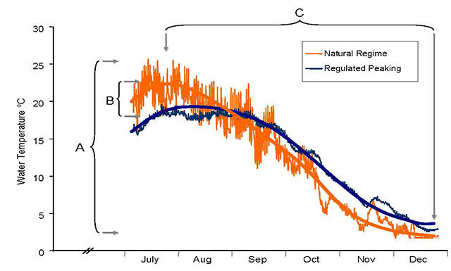
Cold water releases may delay natural seasonal changes in river temperature and reduce the range of temperature variation, both seasonally and diurnally. These alterations to the thermal regime can have consequences for ecosystem condition (Haxton and Findlay 2008; Olden and Naiman 2010) including a reduction in ecosystem productivity and biodiversity, alteration of species’ metabolic rates, interference with breeding cycles, and a decrease in the development and survival of the eggs and larvae of fish and aquatic insects.
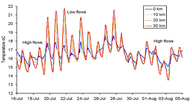
| Dam type | Warmwater River | Coldwater River |
|---|---|---|
| Top draw | Warmer | Much warmer |
| Bottom draw | Much colder | Colder |
Altering temperature can change community composition as thermal limits are reached, alter predation and competition dynamics (Smith 1972), and facilitate the establishment of invasive species (Dunham et al. 2002). Thermal regime alterations may also result in strong compensatory strategies, such as delayed spawning by adults or slowed development by embryos (Olden and Naiman 2010). Changes in fish growth rates can result in biodilution or bioaccumulation of mercury in fish tissue (Simoneau et al. 2005). Warmer winter and spring temperatures from a bottom draw discharge can influence insect growth leading to earlier emergence and increased mortality when the terrestrial environment is snow-covered and weeks away from representing conditions for which the insect are adapted (Raddum 1985). Elevated temperatures decrease the concentration of dissolved oxygen in water while increasing metabolic rates, which may limit the scope of activity (Evans 1990).
Ultimately, the effects of altering water temperature are not straightforward. For example, Holtby (1988) found that logging increased winter water temperature and growth of juvenile salmon. While this alteration might be seen as beneficial, higher growth resulted in earlier outmigration, reduced marine survival, and a reduction in the number of returning spawners.
Large and sudden changes in water temperature (thermopeaking) below dams may cause thermal shock and death in aquatic biota (Donaldson et al. 2008). Evidence suggests the response to thermal shock is highly dependent on the acclimation temperature, the magnitude of the temperature change, and the final endpoint value (Threader and Houston 1983; Thomas et al. 1986; Tang et al. 1987). Sub-lethal effects have also been noted for smaller rates of change, including stress leading to metabolic dysfunction (Wedemeyer 1973), growth inhibition and disease (Wedemeyer and McLeay 1981), and increased predation (Coutant 1973) and polyploidy. Invertebrate drift may increase several fold during 2-4oC changes in temperature during thermopeaking (Carolli et al. 2011). Slower rates of heating or cooling can provide a period of acclimation to facilitate physiological adjustment (McCullough 1999). When flow is low and temperatures are high, hypolimnetic releases during peaking operations can cause rapid and large changes in downstream temperature multiple times per day (Ward and Stanford 1979). When flow is lower at night, as is often the case with peaking waterpower dams, water temperatures will be greater than during the day, which is opposite to the diurnal temperature fluctuations of an natural system (Flodmark et al.2004).
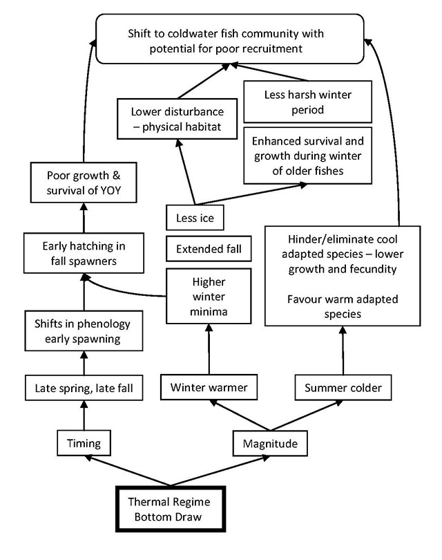
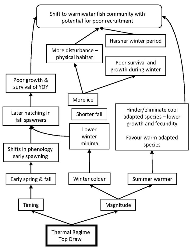
Temperature determines the formation, persistence, and break-up of river ice, which help define the physical character of rivers and fish habitat. Long Canadian winters represent a critical period that heavily impacts overwinter survival and community dynamics of fishes (Cunjak et al. 1998; Scruton et al. 2005). Increased winter temperatures below reservoirs can prevent the formation of ice cover, an effect shown to extend from 5 km (Webb and Walling 1996), 9 km (Ward and Collins 1974), to 32 km from the outlet (Lehmkuhl 1972). In some cases, higher winter temperatures can reduce ice-jam induced flooding, and consequently aquatic habitat availability on the floodplain (Peters and Prowse 2001; Beltaos et al. 2006), limiting ice scouring, resulting in changes to substrate composition and aquatic macrophyte dynamics (Rørslett et al. 1989). In contrast, reducing flow in the winter can result in lower than normal temperatures, increasing the formation of anchor ice and bottom scouring (Ward and Stanford 1979). Super-cooled water supports the formation and accumulation of frazil ice. Frazil ice can have direct deleterious effects on fish by damaging and plugging gill tissues and suffocating fish (Brown et al. 1993). In turbulent water, frazil ice and anchor ice can form to the extent that it occludes the river channel. As anchor ice thickens, it can become buoyant and float away, often taking parts of the substratum with it, including fish eggs. Frazil ice can also accumulate beneath the ice sheet of slower reaches of the river, forming hanging dams, which can fill most of the volume of pools and eliminate living space for fish (Cunjak and Caissie 1993).
In bypassed channels, a reduction of flow can increase water temperatures. The bypass will have less water and riparian vegetation to provide shade, potentially increasing the rate of warming and leading to more extreme temperature ranges.
3.0 Indicator summary
| Characteristic | Indicator |
|---|---|
| Thermal Class | Summer thermal class (June, July and August) |
| Timing | Mean annual date of maxima and minima Monthly modal hour of daily maxima and minima |
| Magnitude | Mean annual maxima and minima Monthly means of daily maxima and minima |
| Variability | Mean annual temperature range Monthly means of daily temperature ranges |
| Rate of Change | Monthly means of daily maximum hourly rates of change |
| Duration | Temperature duration of preferred lethal temperatures |
4.0 Data collection
The ability to capture seasonal and interannual variability in the thermal regime and accurately estimate statistical properties like mean monthly temperature improves as the number of years of data available for analysis increases. It is recognized that the timeframe for the collection of pre-development data are often limited. In these situations, pre-construction data collection over the longest period possible is recommended - ideally a minimum of 2 to 3 years - recognizing that uncertainty increases as the number of years of data decreases.
Temperature loggers should be deployed to provide a continuous measurement of temperature for the entire year. It is recommended that one of the following factors of 60 minutes is used: 5, 10, 15, 20, 30 or 60 minutes, with 30 minutes being preferred since it provides the optimum combination of temporal resolution and logger memory utilization. Longer time intervals may miss daily minima and maxima. It may be advantageous to sample at even shorter intervals (e.g. 15 mins) in small, flashy rivers. To simplify analyses, loggers should be synchronized in time, preferably on the hour or half hour e.g. 13:00, 13:30. For field and laboratory procedures on deploying data loggers, see technical guide by http://www.mnr.gov.on.ca/stdprodconsume/groups/lr/%40mnr/%40aquatics/documents/document/stdprod_068478.pdf [link inactive] (Jones and Allin (2010)).
To capture the within river variation in temperature (natural or existing thermal regime), five data loggers should be placed in the thalweg as noted in Chapter one. Three loggers should be deployed upstream of the in-stream structure past the predicted limit of backwater. If conditions prevent such placement, then three loggers can be placed in a neighbouring natural river with similar physiography and climate. Data from a natural system can be used to separate the effects of annual variability in temperature (hot vs. cold years) from other factors affecting temperature, and assist in yearly comparisons. For existing structures with a reservoir, data loggers should be placed upstream of the maximum extent of the inundation area and five loggers downstream from the structure as described above.
5.0 Thermal regime characteristics, indicators, and assessment criteria
The following sections provide a suite of indicators that can be used to determine thermal characteristics of the ecosystem (Table 2). Each characteristic includes a rationale, description, assessment criteria, and information for evaluating alteration.
Use existing information, if available, to establish an understanding of thermal regime. In many cases information is available but perhaps dated or collected using unidentified means. Traditional ecological knowledge can also help to understand historical and present day characteristics. If appropriate data are not available, or if the available information suggests the medium or high level of alteration, then the collection of field data is recommended to more accurately characterize current conditions.
Most of the indicator metrics and assessment criteria described below can be obtained using the software tool ThermoStat (Jones and Schmidt 2011), which is available online. The recommended methods are written with this in mind; however, all processing steps can be done manually if desired.
5.1 Thermal classification
5.1.1 Description and rationale
Classifying rivers and their reaches by the thermal requirements of fish is a useful preliminary assessment tool. Fish are good integrators of environmental conditions, so the thermal classification of a river is frequently defined by the thermal preferences and tolerances of the fish that inhabit it (i.e. warmwater, coolwater, and coldwater). This provides a simplistic representation of thermal regime. It will not provide information about other ecologically important aspects of temperature such as spatial/temporal variation and rates of change. Caution must be taken, fish and other organisms may exploit or trade-off habitat preferences to minimize the impacts of changing conditions. Migratory species add complexity simply due to their life history. Consider ground truthing by direct sampling of the fish community.
5.1.2 Indicator
Proportion of the temperature record above 25°C (warmwater), between 19-25°C (coolwater), and below 19°C (coldwater) (Coker et al. 2001) during June 1 to August 31.
5.1.3 Information requirements
There are several approaches, qualitative and quantitative, to estimate thermal class including existing knowledge (OMNR and traditional ecological knowledge), existing temperature information, and rapid field techniques described by Stoneman and Jones (1996) (also OSAP Stanfield 2005, and more recently Chu et al. 2009). Direct measures of water temperature following the methods in Jones and Allin ( 2010) collected over 2-3 years likely provides the best approach. Calculate the proportion of the record above 25°C (warmwater), between 19-25°C (coolwater), and below 19°C (coldwater). The proportion of time within each thermal category will help establish a classification. Fish species composition can provide additional support to determine thermal regime e.g. brook trout in abundance suggests a coldwater thermal regime (see Coker et al. 2001); however, there are other drivers of community composition (see Section 6 Biology). Thermal regime prediction is also possible based on landscape characteristics summarized through GIS (percent riparian forest, mean annual air temperature, percent surface water area, and groundwater potential) (Chu et al. 2009).
5.1.4 Assessment criteria
Significant change in the duration in each of the temperature range bins <19°C, 19- 25°C, and >25 °C, relative to the reference or expected condition.
5.1.5 Evaluating alteration
A shift to a different thermal class (<19°C, 19-25°C, and >25°C) is considered a high alteration. The effects of a bottom draw dam will be high in a warm water river. The effects of a top draw dam on a cold water river will also be high. In contrast, the top draw dam may have little effect on a warm water river. Please review introductory sections and see reviews e.g. Clarke et al. (2008). In some rivers, cool thermal refugia such as groundwater seeps might be present which allow coldwater species, e.g. brook trout, to persist during brief periods of high temperatures.
5.1.6 Methods
This classification procedure determines the proportions of temperature measurements greater than 25°C (warmwater), greater than or equal to 19°C and less than or equal to 25°C (coolwater), and less than 19°C (coldwater) (Coker et al., 2001) during June, July and August.
- Collect all records within the period June 1st and August 31st
- Bin records into the three thermal classes of greater than to 25°C, greater than or equal to 19 and less than or equal to 25°C, and proportion less than 19°C.
- Divide the number of records in each thermal class by the total number of records of all three classes (excluding null values) and multiply by 100 to get the percentage of each class.
5.2 Timing
5.2.1 Description and rationale
Water temperatures exhibit seasonal minima and maxima and daily temperature fluctuations that can be significant, particularly on wide and shallow rivers with little groundwater input (Caissie 2006). Most biota inhabiting lotic environments are adapted to diurnal fluctuations in water temperature, which naturally occur on a 24 hour basis (Hubbs 1972) usually reaching a minimum in the early morning hours and a maximum in late afternoon (Caissie 2006). The daily timing of events such as spawning, feeding, hatching and emergence, frequently correspond to these changes in temperature. Artificially stabilizing water temperatures could negatively affect some species whose body processes require a wide daily temperature range for optimal energetic efficiency (Lehmkuhl 1972; Sweeney 1978; Ward and Stanford 1979). For example, spawning fishes and the subsequent emergence and survival of their young, as well as the emergence of benthic invertebrates that may serve as a food source rely on variable temperature. A shift in the annual timing of minimum and maximum temperatures may indicate a shift in the river’s entire thermal profile.
5.2.2 Indicator
Mean annual date of temperature maxima and minima. (Day-of-year, DOY)
5.2.3 Assessment criteria
Assessment criteria include the day-of-years (DOYs) that lie ± 2 weeks and ± 4 weeks from the mean annual date of temperature minima and maxima derived from the reference condition.
5.2.4 Evaluating alteration
The degree of alteration can be determined as follows:
Low alteration: Estimated degree of alteration in mean annual date of temperature min/max is < 2 weeks
Medium alteration: Estimated degree of alteration in mean annual date of temperature min/max is ≥2 weeks and ≤ 4 weeks
High alteration: Estimated degree of alteration in mean annual date of temperature min/max is ≥ 4 weeks
5.2.5 Indicator
Monthly modal hour of daily temperature maxima and minima
5.2.6 Assessment criteria
Assessment criteria include the monthly modal hour of daily maximum and minimum temperature that lie ± 2 hours and ± 6 hours from the monthly modal hour of daily temperature maxima and minima derived from the reference condition.
5.2.7 Evaluating alteration
The degree of alteration can be determined as follows:
Low alteration: Estimated degree of alteration in monthly modal hour of min/max temperature is < 2 hours
Medium alteration: Estimated degree of alteration in monthly modal hour of min/max temperature is ≥ 2 hours and ≤ 6 hours
High alteration: Estimated degree of alteration in monthly modal hour of min/max temperature is > 6 hours
5.2.8 Methods
Annual: This procedure determines a list of the dates of annual maxima and minima for each year within the period of record. The output is a list of minimum and maximum dates for each year of the record in “dd/mm/yyyy” format.
Bin all records into years (one bin for each calendar year). Determine the date of occurrence associated with each bin’s minimum temperature and maximum temperature (a single mean value of these dates can be calculated using the day-of year).
Note: Using partial years that have a large proportion of null data will produce less meaningful results.
Daily: This procedure determines the most common time a stream’s minimum and maximum temperature occur on a daily basis (i.e. daily high and low points in daily temperature). The output is two (i.e. minimum and maximum) modal hours of occurrence for each month.
Bin all record into months (12 bins). Determine the time of occurrence of the daily (midnight to midnight) minimum and maximum for each day within each bin. Days that have no significant troughs or peaks should not be included in the analysis since these will produce unreliable minima/maxima timing results. For example, winter days where temperature hovers around 0°C or cooling/warming trend days where temperature declines/rises steadily from midnight to midnight. Winter days that exhibit near flat-line temperature conditions can be identified as having a daily range of less than 0.25°C. If multiple minima/maxima (troughs/peaks) occur within one day, the lowest/highest minima/maxima should be used to calculate the timing. If minima/maxima include several consecutive equal temperature values (e.g. plateaus) then the earliest time of occurrence should be assigned to that minima/maxima. Bin the gathered times of minima/maxima occurrence for each month into hourly bins (e.g. 13:00 to 13:59, 14:00 to 14:59 etc.) Calculate the mode of all the daily minima and maxima occurrence hours within each monthly bin (i.e. the hourly bin within each month with the most occurrences). If two or more hourly intervals contain equal number of occurrences then the earliest hour interval is reported.
5.3 Magnitude
5.3.1 Description and rationale
Maximum and minimum temperatures provide information on seasonality in temperatures. This information is useful in assessing the shape of the annual pattern of temperature change and is key for defining species’ thermal habitat. Alteration in minimum and/or maximum temperatures can lead to species specific changes in abundance (e.g. loss of warmwater species of fish) and can directly impact survival of aquatic organisms especially for those with narrow temperature preferences (e.g. if a river approaches the upper or lower lethal temperature for a fish species prior to construction, the effects of an in-stream development on the thermal regime become more of a concern especially if the structure limits access to traditional thermal refugia). Temperature also determines the formation, persistence, and break-up of river ice, which help define the physical character of rivers and fish habitat. Winters represent a critical period that heavily impacts survival and community dynamics of fishes (Cunjak et al. 1998; Scruton et al. 2005). In-stream developments can lead to frazil and anchor ice, or prevent the formation of ice cover for several kilometres downstream. Ice dynamics including ice jams, frazil and anchor ice are natural disturbances, like floods, that help maintain biodiversity and for which fishes are adapted.
5.3.2 Indicator
Mean annual temperature maxima and minima
5.3.3 Assessment criteria
Assessment criteria include mean annual minimum and maximum temperatures that lie ±1°C and ±2°C from the mean annual minimum and maximum temperatures derived from the reference condition.
5.3.4 Evaluation alteration
The degree of alteration can be determined as follows:
Low alteration: Estimated degree of alteration is ≤ +1.0° C of mean annual min/max
Medium alteration: Estimated degree of alteration is between +1.0°C - 2.0°C of mean annual min/max
High alteration: Estimated degree of alteration is ≥ +2.0°C of mean annual min/max
5.3.5 Indicator
Monthly means of daily temperature minima and maxima
5.3.6 Assessment criteria
Assessment criteria include mean monthly minimum and maximum temperatures that lie ±1°C and ±2°C from the monthly modal hour of daily temperature maxima and minima, derived from the reference condition.
5.3.7 Evaluating alteration
The degree of alteration can be determined as follows:
Low alteration: Estimated degree of alteration is ≤ +1.0°C of mean monthly temperature min/max
Medium alteration: Estimated degree of alteration is between +1.0°C - 2.0°C of mean monthly temperature min/max
High alteration: Estimated degree of alteration is ≥ +2.0°C of mean monthly temperature min/max
5.3.8 Methods
Annual: This procedure determines the mean annual minimum and maximum temperatures. The output is two values (i.e. averages of all annual minima, averages of all annual maxima). Bin all records into annual bins (one bin for each calendar year) Determine the minimum and maximum temperature value within each bin. Calculate the average of both the minima and maxima within each annual bin.
Daily: This procedure determines the monthly means of daily minimum and maximum temperatures. The output is 24 values: 12 monthly average minima and 12 monthly average maxima. Bin all record into months (12 bins). Determine the daily minimum and maximum for each day within each bin. Days that have no significant troughs or peaks should not be included in the analysis since these will produce unreliable min-max results. For example, winter days where temperature hovers around 0°C or cooling/warming trend days where temperature declines/rises steadily from midnight to midnight. Winter days that exhibit a near flat-line temperature conditions can be identified as having a daily range of less than 0.25°C. If multiple troughs/peaks occur within one day, the lowest/highest troughs/peaks should be used to calculate the mean monthly min/max temperatures. Calculate the average of all the minima and all the maxima.
5.4 Variability
5.4.1 Description and rationale
The daily pattern of water temperature consists of a minimum and a maximum temperature and the pattern resembles a sinusoidal curve. The timing of events such as feeding, hatching and emergence frequently correspond with daily changes in temperature. Most biota inhabiting lotic environments are adapted to diurnal fluctuations in water temperature, which naturally occur on a 24 hour basis (Hubbs 1972), usually reaching a minimum in the early morning hours and a maximum in late afternoon (Caissie 2006). The daily timing of events such as spawning, feeding, hatching and emergence, frequently correspond to these daily changes in temperature. Artificially stabilizing water temperatures could negatively affect some species whose body processes require a wide daily temperature range for optimal energetic efficiency (Lehmkuhl 1972; Sweeney 1978; Ward and Stanford 1979). For example, spawning fishes and the subsequent emergence and survival of their young, as well as the emergence of benthic invertebrates that may serve as a food source rely on variable temperature.
5.4.2 Indicator
Mean Annual Temperature Range
5.4.3 Assessment criteria
Assessment criteria include mean annual temperature range that lie ±1°C and ±4°C from the mean annual temperature range derived from the reference condition.
5.4.4 Evaluating alteration
The degree of alteration can be determined as follows:
Low alteration: Estimated degree of alteration is ≤ +1.0°C of mean annual temperature range
Medium alteration: Estimated degree of alteration is between +1.0°C - 4.0°C of mean annual temperature range
High alteration: Estimated degree of alteration is ≥ +4.0°C of mean annual temperature range
5.4.5 Indicator
Monthly Means of Daily Temperature Range
5.4.6 Assessment criteria
Assessment criteria include monthly mean of daily temperature ranges that lie ± 1°C and ± 4°C from the monthly mean of daily temperature ranges derived from the reference condition.
5.4.7 Evaluating alteration
The degree of alteration can be determined as follows:
Low alteration: Estimated degree of alteration is ≤ +1.0°C of monthly mean of daily temperature range for each month
Medium alteration: Estimated degree of alteration is between +1.0°C - 4.0°C of monthly mean of daily temperature range for each month
High alteration: Estimated degree of alteration is ≥ +4.0°C of monthly mean of daily temperature range for each month
5.4.8 Methods
Annual: This procedure determines the mean annual temperature range. The output is one value representing the average of all annual ranges. Bin all records into years (one bin for each calendar year). Determine the minimum and maximum temperature value for each bin. Calculate the annual temperature range for each bin by subtracting the minimum temperature from the maximum temperature for each bin. Calculate the average of all the annual range values.
Daily: This procedure determines the monthly means of daily temperature ranges. The output is 12 values representing the monthly averages of all daily ranges. For each month, subtract the monthly mean daily minimum from the monthly mean daily maximum to arrive at the monthly mean daily ranges.
Note: because the daily minima and maxima described in section 4.3.8 are used to calculate the monthly means for daily temperature range, the results will reflect the exclusion of days that have no significant troughs or peaks
5.5 Rate of change
5.5.1 Description and rationale
Large and sudden changes in water temperature below in-stream structures can cause thermal shock in aquatic biota (Donaldson et al. 2008). Evidence suggests the response to thermal shock is highly dependent on the acclimation temperature (both constant and cyclic), the magnitude of the temperature shift, and the final endpoint value (Threader and Houston 1983; Thomas et al. 1986; Tang et al. 1987). Sub-lethal effects have also been noted for smaller rates of change including physiological stress leading to metabolic dysfunction (Wedemeyer 1973), growth inhibition and disease initiation (Wedemeyer and McLeay 1981) and increased predation (Coutant 1973). Slower rates of heating or cooling exposure can provide a period of acclimation to facilitate physiological adjustment (McCullough 1999).
5.5.2 Indicator
Monthly Mean of Daily Maximum Hourly Rates of Temperature Change (°C hr-1). This examines the monthly means of daily maximum hourly +/- rates of change for the period of record.
5.5.3 Assessment criteria
Assessment criteria include monthly mean of daily maximum hourly rates of temperature change that lie ± 2°Chr-1 and ± 5°Chr-1 from the monthly mean of daily maximum hourly rates of temperature change derived from the reference condition.
5.5.4 Evaluating alteration
The degree of alteration in the indicator can be determined as follows:
Low alteration: Estimated degree of alteration is ≤ +2.0°C hr-1 relative to the monthly mean of daily maximum hourly rates of temperature change
Medium alteration: Estimated degree of alteration is between +2.0°C hr-1 - 5.0°C hr-1 relative to the monthly mean of daily maximum hourly rates of temperature change
High alteration: Estimated degree of alteration is ≥ +5.0°C hr-1 relative to the monthly mean of daily maximum hourly rates of temperature change.
5.5.5 Methods
This procedure determines the monthly means of daily maximum hourly +/- rates of change for the period of record. The output is 24 values representing the monthly averages of all daily maximum hourly positive and negative rates of change.
- Resample the time series by removing all records with the exception of full hour records (e.g. 12:00:00, 13:00:00, 14:00:00 …).
Note: Do not use hourly averages during resampling.
- Calculate a hourly rate of change value between records by subtracting the next record from the current record (e.g. record (i+1) – record(i)).
Note: Positive rates represent warming rates and negative rates cooling rates.
- Bin all rates according to their sign (2 bins: 1 positive rate bin, 1 negative rate bin).
Note: Zero rates are excluded since they cannot be classified into these bins.
- Bin the records again with the previous bins according to month (24 bins: 12 positive monthly bins, 12 negative monthly bins).
- Calculate the average of each bin.
5.6 Duration
5.6.1 Description and rationale
The thermal characteristics of a stream play an important role in defining the availability of species-specific habitat. Species-specific thermal preferences and tolerances are critical biological elements that define these thermal habitats. Shifting the thermal regime outside a species’ preferred thermal range or beyond its temperature tolerances can lead to changes in community composition and/or the loss of some species.
5.6.2 Indicator
Species-specific temperature duration (+2°C of preferred temperature)
Species-specific temperature duration ≥ lethal temperature during summer period
5.6.3 Assessment criteria
Assessment criteria include species specific temperature duration for preferred and lethal temperatures that lie ±5% and ±10% from the duration of preferred and lethal temperatures derived from the reference condition.
Change in species specific temperature duration ≥ lethal temperatures relative to the reference condition.
5.6.4 Evaluating alteration
The degree of alteration can be determined as follows:
Low alteration: Estimated degree of alteration is ≤ 0–5% of reference condition and/or preferred and lethal temperatures
Medium alteration: Estimated degree of alteration is between > 5 and ≤ 10% of reference condition and/or preferred and lethal temperatures
High alteration: Estimated degree of alteration is ≥ 10% of reference condition and/or preferred and lethal temperatures
5.6.5 Methods
This procedure calculates species-specific temperature durations for the range of +2ºC around the Final Temperature Preferrendum (FTP) and the duration of Upper Incipient Lethal Temperature (UILT) exceedance during the months of June, July and August (i.e. the summer period). The output is two percentage values for each species; one representing the proportion of the summer records that fall within the FTP range and one representing the proportion of summer records that exceed the UILT threshold.
Note: Species-specific temperature values for FTP and UILT are found in Hasnain et al. (2010). If a FTP value is not available, use the Optimum Growth Temperature (OGT) instead. If a UILT value is not available, use the maximum Critical Temperature (CTmax) value instead.
- Collect all records that fall within the period of June 1st and August 31st.
- Using the information from step (a), collect all records that fall within the FTP range of +2°C (inclusive).
- Using the information from step (a), collect all records that are greater than or equal to the UILT threshold.
- Calculate the proportion (%) of the number of summer records within the FTP range to the total number of summer records.
- Calculate the proportion (%) of the number of summer records exceeding the UILT threshold to the total number of summer records.
Chapter 5: Thermal regime - appendix I
Data preparation
The temperature data time series must be processed before performing any calculations. This series of processing steps is necessary to detect any errors and to optimize the time series format for analysis and reporting. Unlike streamflow time series, which are readily available from standardized sources like the Water Survey of Canada, stream temperature data are often collected by individual agencies requiring this data, with no standardized oversight of the collection and reporting process. This often requires stream temperature data to be processed to some degree into a format that is suitable for numerical analysis by “logical” algorithms. It is important to note that although the following indicators can technically be calculated from very few data points, it is highly recommended that no more than 10% of the record be missing (i.e. null data) within each intra-annual analysis period (i.e. seasons and months).
These processing steps may be performed manually. Alternatively, all indicator metrics and assessment criteria can be obtained automatically using the software tool ThermoStat.
Sampling intervals
The data sampling interval determines the temporal resolution of the time series. It is recommended that one of the following factors of 60 minutes is used: 5, 10, 15, 20, 30 or 60 minutes, with 30 minutes being preferred since it provides the optimum combination of temporal resolution and logger memory utilization. Note that if multiple, sequential time series are to be analyzed as a whole they must share a common sampling interval.
Synchronization
The data time stamps must start at a common time on exactly a full hour (e.g. 12:00:00). This makes a direct comparison between multiple time series possible (e.g. from different sampling sites). Ideally, a field data logger should be set up to collect data using this criterion. However, if this is not the case, the time stamps must be synchronized by “rounding” them up or down. In order to minimize the “distance” the time stamps need to be shifted, the shift should be in the direction of the nearest whole multiple of the sampling interval. For example, consider the following series of 30 minute interval data: 12:11:45, 12:41:45, 13:11:45 etc. This should be shifted backward by 11 minutes and 45 seconds to 12:00:00, 12:30:00, 13:00:00 etc Now consider this series: 12:15:00, 12:45:00, 13:15:00 etc. This series sits right on the dividing line between shifting forward or backward. In this type of scenario the times should be shifted backwards to 12:00:00, 12:30:00, 13:00:00, etc. Following this rule will ensure all temperature data are processed in the same way, allowing for more consistent comparisons between data sets. Note that the largest shift introduced using this method will be one half of the sampling interval.
Duplicate records
Data loggers often automatically adjust their time stamps for daylight savings time changes resulting in “duplicate” time stamped records being introduced into the time series. Duplicates must be corrected or deleted.
Below zero days
Negative temperatures are assumed to be the result of less than ideal logger installation, resulting in the logger being embedded in ice during parts of the winter. ThermoStat will accept this data but set these records to 0°C.
Missing records
Missing records are gaps in the data. These gaps must be filled; either by inserting null data, or by another suitable data gap filling technique. When the sampling interval is 60 minutes or less it is possible to estimate single record gaps using linear interpolation of neighbouring data. Gaps longer than one record require more complex gap filling methods.
Leap day records
Temperatures recorded on leap days must be removed to facilitate the numerical analysis of intra-annual time periods of seasons and months. Note that since stream temperatures in Ontario are very likely to be stable (around 0ºC) at the end of February the programming advantages greatly outweigh any disadvantages of removing these “leap” records. Also, removing one day of observations is not likely to impact the analyses from a statistical perspective.
Out-of-water days
Out of water days occur when the water level drops to the point that a logger is exposed to ambient air temperatures. This often results in much larger diel temperature fluctuations than normal for the stream and will adversely affect subsequent analyses. Days with a temperature range exceeding a site dependent threshold can be used to ascertain whether a logger was out-of-water and such days should be removed (i.e. set to null) prior to analysis.
Partial start and end years
Full years of data facilitate partitioning of the time series into seasons and months, which are then analyzed as collections of these periods. For partial start and end years, null records (i.e. no data) serve as placeholders, allowing the time series to remain continuous and permitting the inclusion of these partial years during analysis.
Full leading and trailing year padding
In addition to padding the data to complete partial start and end years it is also necessary to add a full year of null values to the beginning and end of the time series. This is required for analysis of winter seasons that span the end of the calendar year (i.e. December 31). This also allows the autumn season to end before December 31.
Chapter 6: Biology
1.0 Introduction
This chapter describes a process to assess ecosystem change resulting from in-stream development. The data from this process can also be used to monitor ecological characteristics following alteration. The focus in this chapter is on the section of river downstream from an in-stream structure; however, a similar approach and methods can be used in bypassed channels and upstream of the structure. The creation of a reservoir or inundation of a lake is not covered in this chapter.
2.0 Rationale
River ecosystems include a diversity of biotic life that is adapted to the unique dynamics of rivers. Development activities that alter the passage of fish, hydrologic, thermal, chemical, or sediment regimes in rivers will have effects on riverine biota and their habitat. In general, impoundments trap sediments and disrupt the natural process of sediment movement and deposition in the river. In turn, water clarity may increase below dams (Allan and Castillo 2007). Changes to thermal and flow regimes can substantially alter community composition and productivity. Reservoirs typically allow higher levels of primary production than rivers. Organic material trapped in the reservoir releases nutrients and dissolved organic carbon that can lead to large amounts of seston (ultra fine particulate material including phytoplankton and zooplankton). Much of this organic matter drifts downstream of the structure and often feeds a large and productive community of filter feeding invertebrates and fishes. These organisms quickly remove particles, creating a longitudinal (upstream-downstream) gradient in system productivity. In addition to seston, changes in sediment size and water temperature are the primary factors that develop longitudinal zonation (Ward and Stanford 1983). On a temporal scale, the effects of in-stream developments can be immediate (i.e. behavioural responses to flow changes), of moderate term (i.e. changes to biota, communities), and long-term (i.e. geomorphological evolution of the river) (Stoneman 2005).
Many have noted how waterpower facilities affect fish and benthic invertebrates (e.g. Armitage 1984; Dewson et al. 2007; Haxton and Findlay 2008; Murchie et al. 2008). In general, previous studies reported decreases in fish and invertebrate abundance and/or richness and discontinuities in longitudinal zonation (see Ward and Stanford 1979). The response of biota, however, to different in-stream developments and environmental contexts, varies greatly. Fewer studies have focused on the effects of intermittent peaking flows. The addition of other stressors, e.g. invasive species, may confound responses in the dynamics of nutrients and the biological community.
Fish species are often valued ecosystem components (VEC) within rivers and their population status is often a primary socioeconomic interest. However, fish communities depend on the function of lower trophic levels. Primary production supports higher trophic levels by providing food (plants and organic matter) and physical habitat structure. Invertebrates play an essential role in processing and cycling nutrients within ecosystems and pass this energy to fish. The use of single species in assessments, e.g. fish, has been frequently criticized for a lack of comprehensiveness in evaluations of ecosystem condition. Modern monitoring programs have embraced a multi-trophic, ecosystems approach. However, there may also be a need or interest to conduct targeted assessments for VEC species or species at risk.
3.0 Indicator summary
| Characteristic | Indicator |
|---|---|
| Fishes | Fish presence/absence |
| Fishes | Fish community composition Index of abundance for VECs |
| Fishes | Size structure |
| Fishes | Young of the year (YOY) index of abundance; YOY growth |
| Fishes | Methyl mercury in fish tissue |
| Benthos | Composition and abundance of dominant invertebrates (family level) |
| Benthos | Percentage Anisoptera, Plecopter, Trichoptera, Ephemeroptera |
| Basal Resources | Particulate organic matter |
| Basal Resources | Periphyton |
| Basal Resources | Aquatic macrophytes |
4.0 Establishing a reference
In unaltered rivers, current conditions can be used to establish a natural reference for biological indicators but in systems that have already been altered, there will often be insufficient information to do so. As a result, the current condition will serve as the reference condition for assessing potential changes in most biological indicators. Further information on establishing a reference can be found in chapter one, section 3.4.
5.0 Sampling fish
The status of fish and fish populations reflect the health of ecosystems. Fish are relatively long-lived, require distinct habitats during various life history stages, and are generally sensitive to environmental stressors and pollutants and, as such, they integrate the effects of their environment. Many fish occupy high trophic positions, and rely on production in lower trophic levels. As a result, fishes are one of the most commonly used biological indicators in aquatic environments. A variety of species are usually present in freshwater systems, and many species are important for social and economic reasons. It is common to monitor a single fish species of economic or recreational value, or a set of fish community parameters to measure the effects of human alteration on river systems. The environment may affect each life history stage differently.
Spatial considerations
It is important to know what species use the zone of influence, and where and when use happens. Techniques for sampling abiotic and biotic variables in riverine systems are not as well developed as those used in lakes (Flotemersch et al. 2006). While there are few methods for sampling rivers, there are even fewer that specifically address sampling issues in altered rivers where flows fluctuate daily (Jones 2011a, b). In these types of rivers, the lateral areas of riverbed that are routinely wetted and dried create an “intertidal” (Fisher and LaVoy 1972) or varial zone (Lorang et al. 1993). Many have also noted longitudinal gradients in biotic indicators associated with changes in food sources, water temperature, and substrate composition in natural rivers (Vannote et al. 1980; Naiman et al. 1987), altered rivers (Ward and Stanford 1983), and lake outlet systems (Jones 2010). Recognizing the existence and extent of longitudinal and lateral gradients is essential for defining methodological approaches, experimental designs, and the development of monitoring programs.
Temporal considerations
The environmental conditions of rivers are strongly influenced by annual and seasonal variation. Annual variation includes dry and hot years, average years, and wet and cold years. These annual variations in weather can influence fish movement patterns and year-class strength. The seasonality of rivers is well documented. Spring and fall are times of larger flows, colder temperatures, and spawning and overwintering migrations. For example, many tributaries to Lake Superior see thousands of suckers migrate upstream each spring, but by July, most of these rivers are low and contain much fewer fishes. In the fall, many trout, salmon, char, and whitefish ascend these rivers to spawn or overwinter. Observation and sampling only during the summer would result in a large underestimate of use of the river by fishes.
Sampling in rivers can be intimidating and difficult due to the logistical considerations and safety risks associated with high-energy flows. Due to the variability in habitat types, depths, and flow conditions within the zone of influence of a proposed development, a single sampling method is generally not sufficient to provide a representative sample of the community. Professional judgement is required to determine the best suite of methods to measure habitat and sample biota based on the characteristics of the system and the species and life stages sought. The use of standardized techniques is, however, important to provide data that is comparable over time and among systems.
Methods for collecting fish community data in rivers and reservoirs are described in the American Fisheries Society “Standard methods for sampling North American freshwater fishes” (Bonar et al. 2009), the Riverine Index Netting (RIN) manual (Jones and Yunker 2009) and standardized OMNR techniques. Johnson et al. (2007) provide an excellent account of field protocols for sampling salmon and trout in rivers (e.g. boat electrofishing, snorkel surveys).
Electrofishing
Electrofishing using a backpack, shore-side shocking unit or boat are common methods for collecting fishes. Boat electrofishing is possible in deeper rivers with suitable water conductivities and relatively shallow depths (<3m) which allow penetration of the electric field (Carl personal communication). For larger rivers, Jones (http://www.mnr.gov.on.ca/stdprodconsume/groups/lr/%40mnr/%40aquatics/documents/document/stdprod_093462.pdf">2011a [link inactive]) has developed a protocol for sampling the near-shore fish community in wadeable portions of the river. This protocol acknowledges that regulated rivers can have strong longitudinal and lateral gradients in fish abundance that must be considered when developing a sampling plan.
This protocol also works well in rivers with low water conductivity where boat electrofishing is unsuitable. The Ontario Stream Assessment Protocol (OSAP) (Stanfield 2005) incorporates a standard backpack electrofishing procedure for use in wadeable streams (<1m).
Netting protocols
Most netting protocols have been developed for use in lake environments and may present challenges when used in riverine environments due to water flow. The River Index Netting protocol (RIN) is a recommended netting protocol for sampling of fishes in Ontario (Jones and Yunker 2009). The protocol is designed for use in slowly flowing rivers (sections) that cannot be sampled by electrofishing. This net is the same as the North American standard (Bonar et al. 2009), but is shorter in height (0.9m). Research by Jones and Yunker (2011) found that most fish (87%) were captured in the lower half of 1.8-m-high gill nets.
Seining fishes
In shallow (<1.5m), wadeable sections of rivers, beach seining may be used to collect fishes. Seining is a commonly used method in Ontario to sample fish communities in streams. Seining works well for rivers with a slow current and is not recommended in complex environments such as areas with dense aquatic vegetation or large rocky substrate (Freeman et al. 1984). It can be highly variable in capture efficiencies and is not typically as reliable as electrofishing (Poos et al. 2007). However, seining can be a good alternative to electrofishing when there are concerns about the effects of electrofishing on fish populations, especially if species at risk are present (Nielsen 1998). Seining methods can be found in Poos et al. (2007). This method was developed for Ontario streams and includes moving over obstructions in the stream.
Snorkelling
Snorkelling procedures have mainly been developed for use in coldwater rivers and streams. Snorkelling can be applied to streams or rivers that are deep enough to submerge a mask (20cm) and where visibility is not impaired (O’Neal 2007). It is most commonly used to estimate abundance of fish; however, it has been used to sample other characteristics of the community (e.g. habitat use, diversity). Although often selected as the best method to sample salmonids, snorkel surveys have also been used to sample benthic fishes using transects (Magoulick 2004). Use of snorkel surveys as a sampling method can be useful in rivers where conductivity is low or water too deep for electrofishing, or when it may be difficult to use traps or seining (O’Neal 2007). Snorkelling methods can be found in Dunham et al. (2009) and Curry et al. (2009).
Other protocols
Other sampling protocols are available that have not been tested in Ontario or in regulated rivers. For example, Johnson et al. (2007) and Bonar et al. (2009) provide a number of field protocols for sampling fishes in rivers (e.g. redd counts, weirs, larval fish drift nets, and screw-trap, hydroacoustics, aerial fish counts).
6.0 Biological characteristics, indicators, and analyses
The following sections describe a suite of indicators that can be used to determine ecological characteristics of the ecosystem (Table 2). Each indicator includes a rationale for its inclusion in the characterization process, a description of the indicator, and suggested sampling methods. Not all methods are appropriate for all river environments. However, in many cases, the collection of one sample can be used to calculate several indicators. For example, riverine index netting can provide information on presence/absence, community composition, and size structure of fish. In addition, it may be possible to conduct sampling for several indicators concurrently. Recommended analyses for each indicator are also identified in Table 2.
| Characteristic | Indicator | Why | When | Where (Rivers, sites, transects, plots, points) | How | Analyses presentation reporting |
|---|---|---|---|---|---|---|
| Fishes | Fish presence/absence | VEC, use of river | Spring Summer Fall | Presence of fish species in river where and when. At least ten sites (geo- arithmetic spacing). | Various methods | Geo-referenced locations |
| Fishes | Fish community composition: index of abundance for VECs | VEC, use of river, dominance | Aug 15 – Sept 15 | At least ten fixed sites with 3 nets per site | RIN (Jones & Yunker 2011) or shoreline efishing (Jones 2011a) | Index of abundance of each species for each site and year. Non-metric multidimensional scaling (MDS) or correspondence analysis of abundance data. |
| Fishes | Size structure of fish population(fork length mm) | Mortality, growth, recruitment | Aug 15 – Sept 15 | At least ten fixed sites with 3 nets per site | RIN (Jones & Yunker 2011) or shoreline efishing (Jones 2011a) | Size structure of common species for each site and year. |
| Fishes | YOY index of abundance and growth (fork length mm at end of first year of growth) | VEC, recruitment, productivity | Aug 15 – Sept 15 | At least ten fixed sites with 3 plots per site | Shorline efishing (Jones 2011a) | Graph YOY abundance (individual per m2SD) and fork length (mm) of common species distance/site from the in-stream structure. |
| Fishes | Methyl mercury in fish tissue µg/g | Mortality, growth, recruitment | Aug 15 – Sept 15 | Within the reservoir, within 500m of the in-stream structure, and at the end of the ZOI | Various methods | Methyl mercury in fish tissue µg/g by site and year |
| Benthos | Composition and abundance of dominant invertebrates at the family level (individuals per m2) | Productivity, function, health | Aug 15 – Sept 15 | At least ten fixed sites with 3-6 Surber samples per site | Benthic sampling for regulated river (Jones 2011b) | Non-metric multidimensional scaling (MDS) analysis of abundance data. |
| Benthos | Percentage Anisoptera, Plecoptera, Trichoptera, Ephemeroptera | VEC, sentinel species | Aug 15 – Sept 15 | At least ten fixed sites with 3-6 Surber samples per site | Benthic sampling for regulated river (Jones 2011b) | Graph longitudinal relationship between % of each taxa and distance from the instream structure. |
| Basal Resources | Particulate Organic Matter | Ecosystem productivity. Energy pathways to trophic levels | Aug 15 – Sept 15 | At least ten fixed sites with 3-6 samples collected in association with benthic samples | In conjunction with benthos or cores (Jones and Houston 2011). | Graph longitudinal relationship between g/m2 of organics and distance from the in-stream structure. Show SD for each site. |
| Basal Resources | Periphyton | Ecosystem productivity. Energy pathways | Aug 15 – Sept 15 | At least ten fixed sites with 3-6 samples collected in association with benthic samples | Rock scrapes | Graph longitudinal relationship between mg/m2 of periphyton and distance from the in-stream structure. Show SD for each site. |
| Basal Resources | Aquatic Macrophytes | Habitat (e.g. pike), ecosystem productivity | Aug 15 – Sept 15 | 30-40 transects downstream of the in- stream structure in ZOI or aerial imagery. Transects should be frequent enough to represent the river and the patchiness of plants | Transect or imagery | Calculate coverage (m2) for each year. Show imagery for spatial changes i.e. polygon size, locations, and shape. |
6.1 Fish presence and absence
6.1.1 Description and rationale
To accurately understand the ecological characteristics of a river system, its use by fishes must be assessed within the ZOI during spring, summer, and fall. The time when fish traditionally arrive, spawn and disperse must be known. This phenology can also be used in conjunction with thermal regime to predict activities of fish.
6.1.2 Indicator and methods
A list of fish species occupying the portion of the river expected to be influenced by the proposed development. This will include species that use the zone of influence for any portion of their life history throughout the year (e.g. spawning by migratory species) including essential areas such as spawning habitat.
6.2 Fish species index of abundance
6.2.1 Description and rationale
Riverine fish communities typically include a number of species that differ in life histories and habitat requirements for cover, feeding, spawning, and nursery areas, all of which can be affected by changes in the physical and chemical characteristics described in the previous chapters. Ecosystem alterations may result in loss of native fish species, a shift in species composition, or the introduction of non-indigenous species. The assessment and monitoring of fish community composition can provide a more comprehensive indication of ecological condition than any single species. However, there may be interest in collecting information about individual species if they are VECs or species at risk.
6.2.2 Indicator and methods
A list of fish species occupying the ZOI for any portion of their life history throughout the year (e.g. spawning by migratory species) including essential areas such as spawning habitat. Fish community composition is determined by field sampling providing catch per unit effort. Riverine Index Netting and shoreline electrofishing are likely the appropriate sampling methods and can be done singly or together.
6.3 Size structure of fish populations
6.3.1 Description and rationale
The size distribution of fishes is important for understanding growth and recruitment, both of which might be effected by changes in physical and chemical characteristics below in-stream structures. Length frequency distributions provide an important description of population structure.
6.3.2 Indicators and methods
Determine the size structure of fish populations (fork lengths in mm) for VEC, species at risk, or species of interest. Riverine Index Netting and shoreline electrofishing are likely the best sampling methods and can be done singly or together.
6.4 Young of year (YOY) abundance and growth
6.4.1 Description and rationale
Spawning areas and larval and juvenile fish rearing habitat are generally very sensitive to hydrologic alterations associated with in-stream developments. Flow rates can be a trigger for spawning migrations, certain water levels and flows may be necessary to access and utilize spawning habitat, and egg survival within spawning beds is related to water levels and flows. For VEC and SAR species, assessing recruitment and growth of YOY may identify changes in ecological condition and loss of essential habitat earlier than indicators of population structure.
6.4.2 Indicator and methods
Field surveys of YOY abundance as an index or catch per unit effort and size measurements of fish captured in the fall (15 August – 15 September). Sampling at this time will result in measurements representing the majority of growth (fork length mm) for the first year of life. The preferred sampling method is shoreline electrofishing ([link inactive] http://www.mnr.gov.on.ca/stdprodconsume/groups/lr/%40mnr/%40aquatics/documents/document/stdprod_093462.pdf Jones 2011a).
6.5 Mercury in fish tissue
6.5.1 Description and rationale
Mercury is a naturally occurring trace metal typically found in very small quantities in pristine waters. However, the flooding of large areas to create reservoirs can result in conditions which increase the production of the biologically active methyl mercury through increased microbial transformation (methylation) of the inorganic mercury contained in flooded vegetation and soils (Hecky et al. 1991). Mercury originating in a reservoir can be moved downstream and made available for uptake by food webs throughout the ZOI (Rosenberg et al. 1997). Naturally occurring mercury levels and the potential for increased production of methyl mercury are associated with a number of factors and may not be directly related to the area flooded.
Methyl mercury is accumulated in aquatic organisms and because it has a long retention time in animal tissue, biomagnification occurs up the food chain, with predatory fishes such as walleye having the highest mercury concentrations (Jackson 1980). High levels of methyl mercury can affect fish biochemistry, gene transcription, behaviour, reproduction, histology, and growth (Sandheinrich and Miller 2006; Scheuhammer et al. 2007; Drevnick, et al. 2008; Sandheinrich and Wiener 2011). Mercury in fish tissue is also an important concern because of its implications for human consumption.
Because mercury concentrations in water are very small and highly variable, assessment and ongoing monitoring often relies on measurements from fish tissue samples, where bioaccumulation results in higher, more easily measured concentrations.
6.5.2 Indicator and methods
Assess methyl mercury in fish tissue measured in µg/g. If available, existing data on mercury in fish tissue should be used to determine the natural range of variability and to estimate the magnitude of potential changes resulting from construction and operation of the proposed facility. If sufficient data aren’t available or if the available data suggests a moderate to high probability of ecosystem alteration, then field sampling should be done. Field sampling should be done for any development that will create or enlarge an existing reservoir.
Fish samples for mercury analyses should be collected above the predicted limit of backwater due to a reservoir, in the deepest part of the proposed/existing reservoir, within 500 m downstream of the proposed tailrace discharge (MOE), and at the downstream end of the ZOI, and should include:
- One or more species that are sufficiently abundant to ensure capture of a suitable sample size, including:
- young of the year forage fish. Typical species include yellow perch (Perca flavescens) and spottail shiners (Notropis antherinoides). Sampling should be conducted in September, or October if necessary.
- large predatory fish including walleye (Sander vitreus) and northern pike (Esox lucius). Sampling can occur any time during the open-water season.
Tissue sampling protocols for the determination of mercury in tissue from large fish are described in the Ontario Ministry of Environment publication “Protocol for the Collection of Sport Fish Samples for Inorganic and Organic Contaminant Analysis”. MOE should be consulted directly for instructions on sampling forage fish. Tissue analysis should be conducted by a certified laboratory.
6.6 Benthic invertebrates
6.6.1 Description and rationale
Benthic invertebrates are consumers of basal resources (algae, biofilms, organic matter) and secondary consumers. They link basal resources to higher trophic levels, including fishes. Benthic invertebrates are often sampled in aquatic monitoring programs because they are diverse, generally sedentary, and are responsive to environmental alterations. More importantly, they are good indicators of ecosystem productivity and health. In Ontario, there are over 60 species of dragonfly that are provincially rare. Fluctuating flows and changes in course particulate organic matter, thermal regime, sediment dynamics, and water quality can cause changes in the composition and productivity of the invertebrate community.
A number of protocols using benthic invertebrates to assess river health are available but these typically involve many reference rivers and complex statistical analysis (e.g. Environment Canada 2010; Rosenberg et al. 1997; Jones et al. 2004; Barbour et al. 1999; Flotemersch et al. 2006). Most were developed to assess water quality issues, rather than changes in habitat. All protocols provide details on sample design and sampling equipment and methods, as well as data analysis and reporting.
The applicability of the different protocols will depend on site conditions and whether specific biological responses or sentinel species are being investigated. One drawback to these protocols is that they are focussed primarily on small wadeable streams and rivers and may not be suitable for surveying larger non-wadeable rivers. Another is that they describe the composition of the benthic invertebrate community but don’t quantify density or distribution patterns along a river. The latter are important when investigating the effects of water level alterations. The benthic sampling protocol developed by Jones http://www.mnr.gov.on.ca/stdprodconsume/groups/lr/%40mnr/%40aquatics/documents/document/stdprod_093461.pdf (2011b) [link inactive] provides guidance for quantitatively sampling the density and distribution of benthic invertebrates.
Factors such as the type of sampling gear used, habitat types sampled, time of year, level of identification of the biota, and the year that sampling occurred all affect the ability to compare data from different areas. To compare various locations along a river or between rivers, samples should be collected in as short a time frame as possible. The sampling of aquatic invertebrates over a three to four month period compromises the value of comparing data collected at various locations along a river (Fiset 1995).
Quantitative sampling uses a device to sample a known area or volume of habitat. Sampling gear appropriate for the habitat types present are used to obtain biomass or population estimates of the aquatic invertebrate community, as well as information on species composition and species richness. Comparisons of such attributes can only be made when similar sampling gears and effort are used at each location. To account for site variability, replicate sampling is required. To compare quantitative samples between locations, it is necessary to sample similar habitats at each location.
6.6.2 Indicators and methods
Composition and density of invertebrates including sentinel taxa. Data is required on the composition and abundance of the invertebrate community including the percentage Anisoptera, Plecoptera, Trichoptera, Ephemeroptera. Characterization of the community can usually be accomplished with identification to the Family level. Use of the benthic sampling protocol developed by Jones (2011b) is recommended. This method requires sampling each site only once in August and consists of 3-6 Surber samples collected in water 20-30 cm deep during low flow conditions.
6.7 Basal resources
Organic matter, attached algae (periphyton), and aquatic macrophytes provide basal energy sources and critical habitat for many species (e.g. spawning northern pike and macroinvertebrates). In lakes and rivers, macrophytes provide cover for fish and substrate for aquatic invertebrates, produce oxygen, and act as food for some fish and wildlife. Algae and aquatic macrophyte communities respond to water levels, varying flows, water clarity, the timing and frequency of floods. These plants can have both positive and negative effects on the population dynamics of invertebrates and fish. In addition to living plants, particulate organic plant matter such as leaves and dying macrophytes provide food and habitat for many species. In-stream developments can potentially interrupt flow of this organic material and thus change energy flow through the system.
6.7.1 Organic matter
6.7.2 Description and rationale
Dissolved and particulate organic carbon serves as primary food sources for aquatic food webs. Coarse particulate organic matter (CPOM, >1mm), such as leaves and sticks, is the main input into smaller streams, especially in the headwaters (Bilby and Likens 1980). CPOM connects the terrestrial system to the aquatic and once in the stream, it is broken down into smaller fragments by physical and biological processes. CPOM has been shown to correlate with the macroinvertebrate community (Wipfli and Musslewhite 2004) and is the main input of energy to support the food web within the stream. Even small changes in the amount of organic matter entering a river can dramatically affect the composition of fish and invertebrate communities (Moore 1998).
6.7.3 Indicator and methods
Biomass of coarse particulate organic matter. Sampling organic matter requires one site visit and a small amount of laboratory time (see Basal resource sampling protocol Jonesand Houston 2011). Other sampling efforts can be done concurrently.
6.7.4 Periphyton
6.7.5 Description and rationale
Periphyton is a mixture of algae, cyanobacteria, heterotrophic microbes, and detritus attached to submerged surfaces in most aquatic ecosystems. It serves as an important food source for invertebrates, amphibians, and fish. Attached algae responds to changes in water clarity, velocity, depth, nutrients, and the timing and frequency of floods (Biggs 1996). In unshaded streams, periphyton is an important source of energy as it converts sunlight into a food source. At the base of the food web, invertebrates feed on periphyton transferring its energy to higher trophic levels. Although periphyton can have a positive effect on population dynamics, under certain conditions its growth can be too prolific and negatively impact invertebrate and fish communities.
6.7.6 Indicator and methods
Assess the biomass of attached algae. Sampling attached algae requires one site visit and a small amount of laboratory time (see Basal resource sampling protocolJones and Houston 2011). Other sampling efforts can be done concurrently.
6.7.7 Aquatic macrophytes
6.7.8 Description and rationale
Fish use aquatic macrophytes for shelter and refuge and as a place to forage. Macrophytes often enhance diversity in littoral zones by providing structured habitat within the water column and into the substrate, converting light to energy for primary consumers, and influencing nutrient cycling, water quality, water velocities and sedimentation. However, the decomposition of high densities of macrophytes may deplete dissolved oxygen concentrations and cause fish kills (Ploskey 1986). Changes in water flow can affect the distribution of macrophytes, as well as the reverse, with macrophyte distribution influencing water flow (Madsen et al. 2001). Because of this, it is important to get a base-line of macrophytes conditions prior to any in-stream developments.
6.7.9 Indicator and methods
Assess the percentage cover of aquatic macrophytes. Sampling aquatic macrophytes requires one site visit and a small amount of laboratory time (see Basal resource sampling protocol http://www.mnr.gov.on.ca/stdprodconsume/groups/lr/%40mnr/%40aquatics/documents/document/stdprod_093463.pdf Jones and Houston 2011 [link inactive]). Other sampling efforts can be done concurrently.
References
Acres International Limited., 1988a. Streamflow analysis methodology for ungauged small-scale hydro sites in Ontario: Study documentation report. Prepared for Environment Canada Inland Waters Directorate.
Acres International Limited., 1988b. Streamflow analysis methodology for ungauged small-scale hydro sites in Ontario: Applications Manual. Prepared for Environment Canada Inland Waters Directorate.
Acres International Limited., 1994. Hydrologic design methodology for small scale hydro at ungauged sites – Upgrading of Ontario and Atlantic province models. The CANMET Energy Technology Centre (CETC), Energy Technology Branch, Energy Sector, Department of Natural Resources Canada, Ottawa, Ontario.
Ajami, N.K., Gupta, H., Wagener, T. and Sorooshiam, S., 2004. Calibration of a semi- istributed hydrologic model for streamflow estimation along a river system, Journal of Hydrology, 298: 112–135 p.
Alabaster, J. S., and Lloyd, R., 1982. Water quality criteria for freshwater fish. 2nd edition. London, England: Butterworth Scientific. 127-142 p.
Allan J.D. and Castillo, M.M., 2007. Stream Ecology: Structure and Function of Running Waters. 2nd edition. Springer: Dordrecht, Netherlands.
Andrews, E.D., 1980. Effective and bankfull discharges of streams in the Yampa river basin, Colorado and Wyoming. Journal of Hydrology, 46:311-330 p.
Andrews, E.D., 1986. Downstream effects of Flaming Gorge reservoir on the Green River, Colorado and Utah. Geological Society of America Bulletin, 97: 1012-1023 p.
Angradi, T.R., 1999. Fine Sediment and Macroinvertebrate Assemblages in Appalachian Streams: A Field Experiment With Biomonitoring Applications. Journal of the North American Benthological Society, 8(1):49-66 p.
Annable, W.K., 1994. Morphological relations and rural watercourses in southeastern Ontario for use in natural channel design. Masters thesis, University of Guelph, School of Engineering, Guelph, Ontario, Canada.
Annable, W.K., 1996. Morphologic relationships of rural watercourses in Southern Ontario and selected field methods in fluvial geomorphology. Ontario Ministry of Natural Resources, 92 p.
Annear, T., Chisholm, I., Beecher, H., Locke, A., and 12 other authors, 2004. Instream Flows for Riverine Resource Stewardship, revised edition. The Instream Flow Council, Cheyenne, WY., 267-268 p.
Arcement Jr., G.J. and Schneider, V.R., 1989. Guide for selecting Manning’s roughness coefficients for natural channels and flood plains. U.S. Geological Survey Water Supply Paper 2339, 38 p.
Armitage, P.D., 1984. Environmental changes induced by stream regulation and their effect on lotic macroinvertebrate communities. A. Lillehammer and S.J. Saltveit, editors. Regulated Rivers. University of Oslo Press, Oslo, Norway. 139-165 p.
Arnold, J.G., and Allen, P.M., 1999. Automated methods for estimating baseflow and groundwater recharge from stream flow records. J. American Water Resources Association 35 (2): 411-424 p.
Arnwine, D. H., Sparks, K. J., and James, R. R., 2006. Probabilistic monitoring of streams below small impoundments in Tennessee. - Tenn. Dep. Envir. Conserv., Div. Wat. Pollut. Control, Nashville. 282 p.
Arthington, A.H., Bunn, S.E., Poff, N.L., and Naiman, R.J., 2006. The challenge of providing environmental flow rules to sustain river ecosystems. Ecological Applications, 16 (4): 1311- 1318 p.
Auer, N., 1996. Importance of habitat and migration to sturgeons with emphasis on lake sturgeon. Canadian Journal of Fisheries and Aquatic Science 53(Suppl. 1): 152 – 160 p.
Backman, T.W.H. and Evans, A.F., 2002. Gas bubble trauma incidence in adult salmonids in the Columbia River basin. North American Journal of Fisheries Management 22: 579- 584 p.
Backman, T.W.H., Evans, A.F. and Robertson, M.S., 2002. Gas bubble trauma incidence in juvenile salmonids in the Lower Columbia and Snake Rivers. North American Journal of Fisheries Management 22: 965-972 p.
Baldwin, D. S. and Mitchell, A.M., 2000. The effects of drying and re-flooding on the sediment and soil nutrient dynamics of lowland river-floodplain systems. Regulated Rivers Res. Management 16:457-467 p.
Bain, M.B., Harig, A.L., Louks, D.P., Goforth, R.R. and Mills, K.E., 2000. Aquatic ecosystem protection and restoration: advances in methods of assessment and evaluation. Environmental Science & Policy 3: S89-S98 p.
Barbour, M.T., Gerritsen, J., Snyder, B.D., and Stribling, J.B., 1999. Rapid Bioassessment Protocols for Use in Streams and Wadeable Rivers: Periphyton, Benthic Macroinvertebrates and Fish, Second Edition. EPA 841-B-99-002. U.S. Environmental Protection Agency; Office of Water; Washington, D.C.
Barnes Jr., H.A. 1967. Roughness characteristics of natural channels. U.S. Geological Survey Water Supply Paper 1849, 213 p.
Baron, J.S., Poff, N.L., Angermeier, P.L., Dahm, C.N., Gleick, P.H., Hairston, N.G. Jr., Jackson, R.B., Johnston, C.A., Richter, B.D., Steinman, A.D. 2002. Meeting ecological and societal needs for freshwater. Ecological Applications, 12(5): 1247-1260 p.
Bathurst J.C., 1997. Environmental River Flow Hydraulics. in Applied Fluvial Geomorphology for River Engineering and Management (Thorne C. R., Hey R. D. and Newson M. D., eds.), 69-93 p. John Wiley & Sons Ltd., New York.
Bayley, P.B. 1995. Understanding large river-floodplain ecosystems. BioScience 45: 153– 158 p.
Beamesderfer, R.C.P., 1998. Management and trade in Pacific sturgeon. In Proceedings on the Symposium on the Harvest, Trade and Conservation of North American Paddlefish and Sturgeon.[eds.] Williamson, D.F, Benz, G.W. & Hoover, C.M., 95 – 105 p. Chattanooga, TN. TRAFFIC North America/World Wildlife Fund, Washington, DC, USA
Beltaos S, Prowse TD, Carter T., 2006. Ice regime of the lower Peace River and ice-jam flooding of the Peace-Athabasca Delta. Hydrological Processes 20: 4009–4029 p. DOI: 10.1002/hyp.6417
Bergkamp, G., McCartney, M., Dugan, P., McNeely, J., Acreman, M., 2000. Dams, Ecosystem Functions and Environmental Restoration. WCD Thematic Review Environmental Issues II.1. Final Version: November 2000. Prepared for the World Commission on Dams (WSC). 199 p.
Bergström, S., 1976. Development and application of a conceptual runoff model for Scandinavian catchments. SMHI Reports RH0, No. 7, Norrköping.
Bergström, S., 1992. The HBV model - its structure and applications. SMHI Reports RH, No. 4, Norrköping.
Bevelhimer, M.S., 2002. A bioenergetic model for white sturgeon Acipenser transmontanus: assessing differences in growth and reproduction among Snake River reaches. Journal of Applied Ichthyology 18: 550 – 556 p.
Beven, K.J., Kirkby, M.J., Schofield, N., and Tagg, A.F., 1984. Testing a physically-based flood forecasting model (TOPMODEL) for three U.K. Catchments. Journal of Hydrology. 69:119- 143 p.
Bicknell, B.R., Imhoff, J.C., Kittle, J.L., Jr., Donigian, A.S., Jr., and Johanson, R.C., 1997. Hydrological Simulation Program--Fortran, User’s manual for version 11: U.S. Environmental Protection Agency, National Exposure Research Laboratory, Athens, Ga., EPA/600/R-97/080, 755 p.
Biggs, B.J.F., 1996. Hydraulic habitat of plants in streams. Regulated rivers: Research and Management 12: 131-144 p.
Bilby, R.E. and Likens, G.E., 1980. Importance of organic debris dams in the structure and function of stream ecosystems. Ecology 61: 1107-1113 p.
Boers, P.C.M., 1991. The influence of pH on phosphate release from lake sediments. Water Res. 25: 309-311 p.
Boers, P.C.M., and Van Hese, O., 1988. Phosphate release from the peaty sediments of the Loosdrecht Lakes (The Netherlands). Water Res. 22: 355-363 p.
Bonar, S.A., Hubert, W.A., and Willis, D.W., editors. 2009. Standard Methods for Sampling North American Freshwater Fishes. American Fisheries Society, Bethesda, Maryland.
Bouck, G. R., 1980. Etiology of Gas Bubble Disease. Transactions of the American Fisheries Society 1980; 109: 703-707 p.
Bowen, Z.H., Bovee, K.D. and Waddle, T.J., 2003. Effects of flow regulation on shallow water habitat dynamics and floodplain connectivity. Transactions of the American Fisheries Society. 132: 809-823 p.
Brandt, A.S., 2000. Classification of geomorphological effects downstream of dams. Catena, 40: 375-401p.
Brett, J.R., 1971. Energetic responses of salmon to temperature: a study of some thermal relations in the physiology and freshwater ecology of sockeye salmon (Oncorhynchus nerka). American Zoology 11: 99–113 p.
Brilly, M., Kobold, M., and Vidmar, A., 1997. Water information management system and low flow analysis in Slovenia. FRIEND '97 - Regional Hydrology: concepts and models for sustainable water resource management. Proceedings from the International Conference, 246:117-124 p.
British Columbia Ministry of Environment, 1997. Ambient Water Quality Criteria for Dissolved Oxygen.
Broman, D., Naf, C., Axelman, J., Bandh, C., Pettersen, H., Johnstone, R. and Walberg, P., 1996. Significance of bacteria on marine waters for the distribution of hydrophobic organic contaminants. Environmental Science and Technology 30(4):1238-1241 p.
Brookes, A., 1988. Channelized Rivers: Perspectives for Environmental Management. John Wiley. New York
Brown, C., and King, J., 2000. Environmental Flow Assessments for Rivers. A summary of the DRIFT process. Southern Waters Information Report No 01/00, 26 p.
Brown, D.R., 2007. Freshwater fish in Ontario’s Boreal: Status, conservation and potential impacts of development. WCS Canada Conservation Report No. 2. 98 p.
Brown, R.S., Stanislawski, S.S., Mackay, W.C., 1993. Effects of frazil ice on fish. In Proceedings of the Workshop in Environmental Aspects of River Ice, Prowse TD (ed). NHRI Symposium Series No. 12, National Hydrology Research Institute, Saskatoon, Canada; 261-278 p.
Brune, G.M., 1953. Trap Efficiency of Reservoirs. Transactions of the American Geophysical Union, 34(3), 407-418 p.
Bunn, S.E. and Arthington, A.H., 2002. Basic principles and ecological consequences of altered flow regimes for aquatic biodiversity. Environmental Management, 30(4): 492-507 p.
Bunte, K., Swingle, K.W. and Abt, S.R., 2007. Guidelines for using bedload traps in coarse- bedded mountain streams: construction, installation, operation, and sample processing. United State Department of Agriculture Forest Service, Rocky Mountain Research Station, General Technical Report RMRS-GTR-191. 91p.
Bushaw K.L., Zepp, R.G., Tarr, M.A., Schulz-Jander, D., Bourbonniere, R.A., Hodson, R.E., Miller, W.L., Bronk, D.A., and Moran, M.A.,1996. Photochemical release of biologically labile nitrogen from aquatic dissolved organic matter. Nature 381. 404-407p.
Caissie, D. 2006. The thermal regime of rivers: a review. Freshwater Biology 51: 1389- 1406. DOI: 10.1111/j.1365-2427.2006.01597.x
Canadian Council of Ministers of the Environment. 1999a. Canadian water quality guidelines for the protection of aquatic life: Dissolved gas supersaturation. In: Canadian environmental quality guidelines, 1999, Canadian Council of Ministers of the Environment, Winnipeg.
Canadian Council of Ministers of the Environment. 1999b. Canadian water quality guidelines for the protection of aquatic life: Dissolved oxygen (freshwater). In: Canadian environmental quality guidelines, 1999, Canadian Council of Ministers of the Environment, Winnipeg.
Canadian Council of Ministers of the Environment. 2002. Canadian water quality guidelines for the protection of aquatic life: Total particulate matter. In: Canadian environmental quality guidelines, 1999, Canadian Council of Ministers of the Environment, Winnipeg.
Canadian Council of Ministers of the Environment. 2003a. Canadian water quality guidelines for the protection of aquatic life: Guidance on the Site-Specific Application of Water Quality Guidelines in Canada: Procedures for Deriving Numerical Water Quality Objectives. In: Canadian environmental quality guidelines, 1999, Canadian Council of Ministers of the Environment, Winnipeg.
Canadian Council of Ministers of the Environment. 2003b. Canadian water quality guidelines for the protection of aquatic life: Inorganic mercury and methylmercury. In: Canadian environmental quality guidelines, 1999. Canadian Council of Ministers of the Environment, Winnipeg.
Canadian Council of Ministers of the Environment. 2003c. Canadian water quality guidelines for the protection of aquatic life: Nitrate Ion. In: Canadian environmental quality guidelines, 1999, Canadian Council of Ministers of the Environment, Winnipeg.
Canadian Council of Ministers of the Environment. 2004. Canadian water quality guidelines for the protection of aquatic life: Phosphorus: Canadian Guidance Framework for the Management of Freshwater Systems. In: Canadian environmental quality guidelines, 2004, Canadian Council of Ministers of the Environment, Winnipeg.
Canadian Council of Ministers of the Environment. 2007. Canadian water quality guidelines for the protection of aquatic life: Nutrients. In: Canadian environmental quality guidelines, 1999, Canadian Council of Ministers of the Environment, Winnipeg.
Canadian Council of Ministers of the Environment. 2010. Canadian water quality guidelines for the protection of aquatic life: Ammonia. In: Canadian environmental quality guidelines, 1999, Canadian Council of Ministers of the Environment, Winnipeg.
Canadian Council of Ministers of the Environment. 2011. Protocols Manual for Water Quality Sampling in Canada.
Carling, P.A., 1988. The concept of dominant discharge applied to two gravel-bed streams in relation to channel stability thresholds. Earth Surface Processes and Landforms, 13:355- 367 p.
Carlisle, D.M., Wolock, D.M., and Meador, M.R., 2010. Alteration of streamflow magnitudes and potential ecological consequences: a multiregional assessment. Frontiers in Ecology and the Environment 2010; DOI: 10.1890/100053.
Carolli M., Bruno M.C., Siviglia A., Maiolini B., 2011. Responses of benthic invertebrates to abrupt changes of temperature in flume simulations. River Research and Applications. DOI: 10.1002/rra.1520
Carpenter, T.M. and Georgakakos, K.P., 2006. Intercomparison of lumped versus distributed hydrologic model ensemble simulations on operational forecast scales. Journal of Hydrology, 1-2: 174-185 p.
Cavanagh, N.S., Nordin, R.N., Pommen, L.W. and Swain, L.G., 1998a. Guidelines for Designing and Implementing a Water Quality Monitoring Program. British Columbia Ministry of Environment, Lands and Parks.
Cavanagh, N.S., Nordin, R.N., Pommen, L.W. and Swain, L.G., 1998b. Guidelines for Interpreting Water Quality Data. British Columbia Ministry of Environment, Lands and Parks.
Chang, C., Ashenhurst, F., Damaia, S. and Mann, W., 2002. Ontario Flow Assessment Techniques, Version 1.0. OMNR, Northeast Science & Information, South Porcupine, Ontario.
Chapman, D. and Kimstach, V., 1996. Selection of Water Quality Variables in Water Quality Assessments - A Guide to Use of Biota, Sediments and Water in Environmental Monitoring - Second Edition. Chapman, D. (editor). University Press, Cambridge
Chapman, T.G., 1999. A comparison of algorithms for stream flow recession and baseflow separation. Hydrological Processes, 13: 701–714 p.
Chorley, R.J., Schumm, S.A., Sugden, D.E. 1984. Geomorphology. Methuen, New York. 605 p.
Chu, C., Jones, N.E., Piggott, A.R., Buttle, J.M., 2009. Evaluation of a simple method to classify the thermal characteristics of streams using a nomogram of daily maximum air and water temperatures. North American Journal of Fisheries Management 29: 1605–1619 p. DOI: 10.1577/M08-251.1
Church, M., Ham, D., Hassan, M., Slaymaker, O., 1999. Fluvial clastic sediment yield in Canada: scaled analysis. Canadian Journal of Earth Science, 36: 1267-1280 p.
Church, M., 2002. Geomorphic threshold in riverine landscapes. Freshwater Biology 47: 541-557 p.
Clarke, K.D., Pratt, T.C., Randall, R.G., Scruton, D.A., Smokorowski, K.E., 2008. Validation of the flow management pathway: effects of altered flow on fish habitat and fishes downstream from a hydropower dam. Canadian Technical Report of Fisheries and Aquatic Sciences 2784, Ottawa, Canada; 111.
Clarke, R.T., 1990. Bias and variance of some estimators of suspended sediment load, Hydrological Sciences Journal, 35(3): 253-261 p.
Coker, G.A., Portt, C.B., Minns, C.K., 2001. Morphological and ecological characteristics of Canadian freshwater fishes. Canadian Manuscript Report of Fisheries and Aquatic Sciences 2555, Ottawa, Canada; 89. http://dsp-psd.pwgsc.gc.ca/collection_2007/dfo-mpo/Fs97-4-2554E.pdf [link inactive] [22 November 2011].
Coleman, W.G., 1996. Biodiversity and industry ecosystem management. Environ. Manage. 20: 815-825 p.
Collier, M., Webb, R.H., and Schmidt, J.C., 1996. Dams and Rivers, Primer on the Downstream Effects of Dams. U.S. Geological Survey Circular 1126, 94 p.
Coutant, C.C., 1973. Effect of thermal shock on vulnerability of juvenile salmonids to predation. Journal of the Fisheries Research Board Canada 30: 965-973 p.
Covich, A.P., Clements, W.H., Fausch, K.D., Stednick, J.D., Wilkens-Wells, J., Abt, S.R., 2005. Ecological Integrity and Western Water Management: A Colorado Perspective. Water in the balance No. 3. Colorado Water Resources Research Institute. 25 p.
Cunjak, R.A., Caissie, D., 1993. Frazil ice accumulation in a large salmon pool, in the Mirimichi River, New Brunswick: ecological implications for overwintering fish. In Proceedings of the Workshop in Environmental Aspects of River Ice, Prowse TD (ed). NHRI Symposium Series No. 12, National Hydrology Research Institute, Saskatoon, Canada; 279-295 p.
Cunjak, R.A., Prowse, T.D., Parrish, D.L., 1998. Atlantic salmon Salmo salar in winter:"the season of parr discontent"? Canadian Journal of Fisheries and Aquatic Sciences 55: 161- 180 p.
Curry, R.A., Hughes, R.M., McMaster, M.E. and Zafft, D.J., 2009. Coldwater fish in rivers. 139-154p. in S.A. Bonar, W.A. Hubert, and D.W. Willis, editors. Standard Methods for Sampling North American Freshwater Fishes. American Fisheries Society, Bethesda, Maryland.
Curtis, K.E., Renshaw, C.E., Magilligan, F.J., Dade, W.B., 2010. Temporal and spatial scales of geomorphic adjustments to reduced competency following flow regulation in bedload-dominated systems. Geomorphology, 118(1-2): 105-117 p.
Dade, W.B., Renshaw, C.E. and Magilligan, F.J., 2011. Sediment transport constraints on river response to regulation. Geomorphology, 126: 245-251 p.
Danish Hydraulic Institute (DHI). 1998. MIKE SHE Water Movement - User Guide and Technical Reference Manual, Edition 1.1.
Davies, S.P. and Jackson, S.K., 2006. The biological condition gradient: A descriptive model for interpreting change in aquatic ecosystems. Freshwater Bioassessment 16: 1251
Department Of Water Affairs And Forestry (DWAF), 1999. Resource directed measures for Protection of water resources. Volume 3. River ecosystems. Version 1.0. Department of Water Affairs and Forestry, Pretoria.
Dewson, Z.S., James, A.B.W., and Death, R.G., 2007. A review of the consequences of decreased flow for instream habitat and macroinvertebrates. Journal of the North American Benthological Society 26: 401-415 p.
Dickinson, W.T., 1981. Accuracy and precision of suspended sediment loads. In: Erosion and Sediment Transport Measurement (Proc. Florence Symp. June 1981) 195-202 p. IAHS Publ. no. 133.
Dillon, P.J. and Molot, L.A., 1997. Dissolved organic and inorganic carbon mass balances in central Ontario lakes. Biogeochem. 36:29-42 p.
Dingman, S.L., 1994. Physical Hydrology. New York: MacMillan Publishing Company, 575 p.
Donaldson M.R., Cooke S.J., Patterson D.A., Macdonald J.S., 2008. Cold shock and fish. Journal of Fish Biology 73: 1591-1530. DOI: 10.1111/j.1095-8649.2008.02061.x
Doudoroff, P. and Shumway, D.I., 1970. Dissolved oxygen requirements of freshwater fishes. F.A.O. Fish. Tech. Pap. 86. 291 p.
Drevnick, P.E., Roberts, A.P., Otter, R.R., Hammerschmidt, C.R., Klaper, R., and Oris, J.T.,2008. Mercury toxicity in livers of northern pike (Esox lucius) from Isle Royale, USA. Comp. Biochem. Physiol. Part C 147:331–338 p.
Dunham J.B., Adams S.B., Schroeter R.E., Novinger D.C., 2002. Alien invasions in aquatic ecosystems: toward an understanding of brook trout invasions and potential impacts on inland cutthroat trout in western North America. Reviews in Fish Biology and Fisheries 12: 373-391. DOI:10.1023/A:1025338203702
Dunham, J.B., Rosenberger A.E., Thurow R.F., Dolloff C.A., and Howell, P.J., 2009. Coldwater fish in wadeable streams. Pages 119-138 in S.A. Bonar, W.A. Hubert, and D.W. Willis, editors. Standard Methods for Sampling North American Freshwater Fishes. American Fisheries Society, Bethesda, Maryland.
Dunne, T., and Leopold, L.B., 1978. Water in environmental planning. San Franscisco, CA: W.H. Freeman and Co., 181 p.
Dury, G.H., Hails, J.R. and Robbie, M.B., 1963. Bankfull discharge and the magnitude- frequency series. Australian Journal of Science, 26:123-124.
Dury, G.H., 1973. Magnitude-frequency analysis and channel morphology, In: Morisawa, M. (ed), Fluvial Geomorphology, SUNY Binghamton, Publications in Geomorphology, 91- 121 p. -1266
Eaton, A.D., Clesceri, L.S., Rice, E.W., Greenberg, A.E., and Franson (ed.), M.A.H., 2005. Standard methods for the examination of water and wastewater, 21st ed. American Public Health Association, Washington, DC.
Ebersole, J.l., Liss, W.J. and Frissel, C.A., 2001. Relationship between stream temperature, thermal refugia and rainbow trout, Oncoryhnchos mykiss abundance in arid-land streams in the northwestern United States. Ecology of Freshwater Fish 10:1-10 p.
Eckhardt, K., 2008. A comparison of baseflow indices, which were calculated with seven different baseflow separation methods. Journal of Hydrology, 352: 168-173 p.
Edwards, T.K. and Glysson, G.D., 1999. Field methods for measurement of fluvial sediment: U.S. Geological Survey Techniques of Water-Resource Investigations. Book 3, Chapter C2. (http://water.usgs.gov/pubs/twri/twri3-c2/pdf/TWRI3-C2.pdf) [link inactive]
EPA, 1997. Hydrological Simulation Program – Fortran (HSPF). United States Environmental Protection Agency.
Environment Canada., 2010. Canadian Aquatic Biomonitoring Network: Wadeable Streams Field Manual. 52 pp.
Environmental Protection Agency., 2003. Multimedia, multipathway, and multireceptor risk assessment (3MRA) modeling system, Volume I: modeling system and science. SAB Review Draft [EPA530-D-03-001a].
ESSA, Technologies Ltd. 2005. Ecological indicators for effectiveness monitoring for water management planning. ESSA Technologies Limited, 11 Angelica Avenue, Richmond Hill, Ontario. 18 pp.
Eziashi, A.C., 1999. An appraisal of the existing descriptive measures of river channel patterns. Journal of Environmental Sciences 3(2): 253-257.
Evans, D.O., 1990. Metabolic thermal compensation by rainbow trout: effects on standard metabolic rate and potential usable power. Transactions of the American Fisheries Society 119: 585-600.
Ferguson, R.I., 2005. Estimating critical stream power for bedload transport calculations in gravel-bed rivers. Geomorphology 70: 33-41.
Fiset, W., 1995. A review of aquatic invertebrate studies conducted in the Moose River Basin. OMNR, Northeast Science and Technology. TR-024. 60pp.
Fisher, S.G. and LaVoy, A., 1972. Differences in littoral fauna due to fluctuating water levels below a hydroelectric dam. Journal of the Fisheries Research Board of Canada 29: 1472-1476.
Flodmark, L.E.W., Vøllestad, L.A., Forseth, T., 2004. Performance of juvenile brown trout exposed to fluctuating water level and temperature. Journal of Fish Biology 65: 460-470. DOI: 10.1111/j.0022-1112.2004.00463.x
Flotemersch, J.E., Stribling, J.B., and Paul, M.J., 2006. Concepts and Approaches for the Bioassessment of Non-wadeable Streams and Rivers. EPA 600-R-06-127. US Environmental Protection Agency, Cincinnati, Ohio.
Flügel, W.A., and Lüllwitz, T.H., 1993. Using a distributed hydrologic model with the aid of GIS for comparative hydrological modelling of micro – and mesoscale catchments in the USA and in Germany. Macroscale Modelling of the Hydrosphere. Proceedings of the Yokohama Symposium, July 1993. IAHS Publication No. 214: 59-66 p.
Freeman, B.J., Greening, J.S., and Oliver, J.D., 1984. Comparison of three methods for sampling fishes and macroinvertebrates in a vegetated freshwater wetland. Freshwater Ecology2: 603–609 p.
Friedl, G., and Wüest, A., 2002. Disrupting biogeochemical cycles - Consequences of damming. Aquatic Sciences 64: 55–65.
Fukushima, M., 2001. Salmonid habitat-geomorphology relationships in low-gradient streams. Ecology, 82: 1238-1246.
Galster, J.C., Pazzaglia, F.J., Hargreaves, B.R., Morris, D.P., Peters, S.C., Weisman, R.N., 2006. Effects of urbanization on watershed hydrology: The scaling of discharge with drainage area. Geology, 34(9): 713-716 p.
Galster, J.C., 2007. Natural and anthropogenic influences on the scaling of discharge with drainage area for multiple watersheds. Geosphere, 3(4): 260-271 p.
Gassman, P.W., Reyes, M.R., Green, C.H., and Arnold, J.G., 2007. The Soil and Water Assessment Tool: Historical development, applications, and future research directions. Transactions of the ASABE, 50(4): 1211-1250 p.
Gergel, S.E., Turner, M.G., and Kratz, T.K., 1999. Dissolved organic carbon as an indicator of the scale of watershed influence on lakes and rivers. Ecological Applications, 9(4), 1377– 1390 p.
Gleick, P.H., 1992. Environmental consequences of hydroelectric development: The role of facility size and type. Energy, 17(8): 735-747 p.
Goldstein, R.M., Wang, L., Simon, T.P., Stewart, P.M., 2002. Development of a stream habitat index for the Northern Lakes and Forests Ecoregion. North American Journal of Fisheries Management, 22: 452-464 p.
Gomez, B., and Church, M., 1989, An assessment of bed load sediment transport formulae for gravel bed rivers. Water Resources Research, 25:. 1,161–1,186 p.
Gordon, N.D., McMahon, T.A., Finlayson, B.L., Gippel, C.J., and Nathan, R.J., (eds.), 2004. Stream Hydrology, An Introduction for Ecologists. 2nd edition., John Wiley & Sons, 429 p.
Graf, W.L., 2006. Downstream hydrologic and geomorphic effects of large dams on American rivers. Geomorphology, 79: 336-360 p.
Grant, G.E., Duval, J.E., Koerper, G.J, and Fogo, J.L., 1992. xspro: a channel cross- section analyzeer. In Dodson and Associates, Inc., Hydro-CD 6th Edition.
Grant, G.E., Schmidt, J.C. and Lewis, S.L., 2003. A geological framework for interpreting downstream effects of dams on rivers; A Unique River; Water Science and Application 7; American Geophysical Union; 209-225 p.
Hasnain, S.S., Minns, C.K., Shuter, B.J., Birk-Urovitz, E., Birk-Urovitz, A., 2010. Compilation of Ecological Temperature Metrics for Canadian Freshwater Fishes. Climate Change Research Report CCRR-17, Ontario Ministry of Natural Resources; 55.
Halleraker, J.H., Alfredsen, K., Arnekleiv, J.V., Fjeldstad, H.P., Harby, A., and Saltveit, S.J. ,1999. Environmental impacts of hydro peaking with emphasis on river Nidelva in Trondheim, Norway. Paper presented at the International Seminar “Optimum use of run-of- river hydropower schemes, 21–23 June, Trondheim, International Center for Hydropower, 7 p.
Harby, A., Halleraker, J.H., Alfredsen, K., Arnekleiv, J.V., Johansen, S., Saltveit, S.J., 1999. Impacts of hydropeaking on Norwegian riverine ecosystems. Proceedings of the 3rd International Symposium of Ecohydraulics. Salt Lake City, USA. 12-16 July.
Harman, C. and Stewardson, M., 2005. Optimizing dam release rules to meet environmental flow targets. River Research and Applications, 21:113-129 p.
Hauer, F. P. and Hill, W.R., 2007. Temperature Light and Oxygen. In Methods in Stream Ecology, Second Edition, 2007, Edited by Hauer, F. R. and G. A. Lamberti. Academic Press, Burlington, MA, USA. 103-118 p.
Haxton, T.J., Findlay C.S., 2008. Meta-analysis of the impacts of water management on aquatic communities. Canadian Journal of Fisheries and Aquatic Sciences 65: 437-447, 537-557 p. DOI: 10.1139/F07-175
Hayes, D.C., and Nelms, D.L., 2001. Base-flow characteristics of streams in the Valley and Ridge, Blue Ridge, and Piedmont Physiographic Provinces of Virginia and other Mid-Atlantic states. U.S. Geological Survey, Appalachian Region Integrated Science Workshop Proceedings, Open-File Report 01-406, Gatlinburg, Tennessee, October 22-26, 2001.
Hecky, R.E., Ramsay, D.J., Bodaly, R.A. and Strange, N.E., 1991. Increased methymercury contamination in fish in newly formed freshwater reservoirs. In Advances in mercury toxicology. Edits by T. Suzuki, N. Imura and T. W. Clarkson. Plenum, New York. 33-52 p.
Hicks, D.M, and Gomez, B. 2003. Sediment Transport, pp: 425-461, In: G.M. Kondolf and H. Piégay, (Eds), Tools in Fluvial Geomorphology. Wiley, Chichester, 688 p.
Holling, C.S. 1973. Resilience and stability of ecological systems. Ann. Rev. Ecol. Syst. 4:1-23
Holtby, L.B., 1988. Effects of logging on stream temperatures in Carnation Creek, British Columbia, and associated impacts on the coho salmon (Oncorhynchus kisutch). Canadian Journal of Fisheries and Aquatic Sciences 55: 502–515 p.
Hubbs, C., 1972. Some thermal consequences of environmental manipulations of water. Biological Conservation 4: 185-188 p.
Hudson, J.J., Taylor, W.D., and Schindler, D.W., 2000. Phosphate concentrations in lakes. Nature: 406:54-56 p.
Jackson, T., 1980 Mercury speciation and distribution in a polluted river-lake system as related to the problems of lake restoration. In: Proceedings of the International Symposium for Inland Waters and Lake Restoration. United States Environmental Protection Agency/Organisation for Economic Cooperation and Development, Portland, Maine, 93-101 p.
Jones, N.E., Allin, L., 2010. Measuring Stream Temperature Using Data Loggers: Laboratory and Field Techniques. Ontario Ministry of Natural Resources, Aquatic Research and Development Section, 29 p.
Jones, N.E., Schmidt, B., 2011. ThermoStat: Tools for Analyzing Thermal Regimes Reference Manual Version 3. Ontario Ministry of Natural Resources, Aquatic Research and Development Section, River and Stream Ecology Lab.
Huggett, R.J., 2007. Fundamentals of Geomorphology. Routledge, London, UK. 400 p. Hughes, D.A. and Smakhtin, V.Y., 1996. Daily flow time series patching or extension: A spatial interpolation approach based on flow duration curves. Hydrological Sciences, 41(6):851-871 p.
Jinfa, L. and Xiuhua, H., 2004. The relationship between sediment yield and catchment characteristics in the middle Yellow River basin of China. Sediment Transfer through the Fluvial System (Proceedings of a symposium held in Moscow, August 2004. IAHS Publ. 288: 212-219 p.
Johnson, D.H., Shrier, B.M., O’Neal, B.S., Knutzen, J.A., Augerot, X., T.A., O’Neil et al. 2007. Salmonid Field Protocols Handbook: Techniques for Assessing Status and Trends in Salmon and Trout Populations. American Fisheries Society, Bethesda, Maryland. 478 p.
Johnson, W.C., 2002. Riparian vegetation diversity along regulated rivers: contribution of novel and relict habitats. Freshwater Biology 47: 749-759 p.
Jones, C., Somers, K.M., Craig, B., and Reynoldson, T., 2004. Ontario Benthos Biomonitoring Network Protocol Manual, Version 1.0. Ontario Ministry of Environment.
Jones, N.E., 2010. Incorporating Lakes within the River Discontinuum: Longitudinal Changes in Ecological Characteristics in Stream-Lake Networks. Canadian Journal of Fisheries and Aquatic Sciences 67: 1350-1362 p.
Jones, N.E., 2011a. Electrofishing Rivers: Nearshore Community. Sampling Methodologies for Ontario’s Flowing Waters. Ontario Ministry of Natural Resources, Aquatic Research and Development Section, River and Stream Ecology Lab, Aquatic Research Series 2011-06
Jones, N.E., 2011b. Benthic Sampling in Natural and Regulated Rivers. Sampling Methodologies for Ontario’s Flowing Waters. Ontario Ministry of Natural Resources, Aquatic Research and Development Section, River and Stream Ecology Lab, Aquatic Research Series 2011-05
Jones, N.E. and Yunker, G., 2009. Riverine Index Netting Manual of Instructions. Ontario Ministry of Natural Resources, River and Stream Ecology Unit. 29 p.
Jones, N.E. and Yunker, G., 2011. Development of a Riverine Index Netting Protocol: Comparisons of Net Orientation, Height, Panel Order, and Line Diameter. North American Journal of Fisheries Management 31:23–31 p.
Jones, N.E. and Houston, B.E., 2011. Basal Resources Sampling in Rivers. Sampling Methodologies for Ontario’s Flowing Waters. Ontario Ministry of Natural Resources, Aquatic Research and Development Section, River and Stream Ecology Lab, Aquatic Research Series 2011-07.
Junk, W.J., Bayley, P.B., and Sparks, R.E., 1989. The flood pulse concept in river floodplain systems. Can. J. Fish. Aquat. Sci. Spec. Publ. 106:110-127 p.
Kannel, P.R., Kanel, S.R., Lee, S., Lee, Y.S., and Gan, T.Y., 2011. A Review of Public Domain Water Quality Models for Simulating Dissolved Oxygen in Rivers and Streams Environmental Modelling and Assessment 16(2): 183-204 p.
Karr, J.R., 1991. Biological Integrity: A long-neglected aspect of water resource management. Ecological Applications 1(1): 66-84 p.
Karr, J.R., 1999. Defining and measuring river health. Freshwater Biology 41, 221-234 p. King, J., Brown, C. and Sabet, H., 2003. A scenario-based holistic approach to environmental flow assessments for rivers. River Research and Applications 19: 619-639 p.
King, J. and Louw, D., 1998. Instream flow assessments for regulated rivers in South Africa using the Building Block Methodology. Aquatic Ecosystem Health and Management, 1: 109-124 p.
Knighton, D., 1998. Fluvial Forms and Processes, A New Perspective. John Wiley & Sons, New York, 383 p.
Kondolf, G.M., and Piégay, H.((eds)), 2003. Tools in Fluvial Geomorphology. Wiley, Chichester, 688 p.
Kondolf, G.M., Lisle, T.E, Wolman, G.M., 2003. Bed sediment measurement. Chapter 13 In G. M. Kondolf and H. Piégay, (Eds.). Tools in fluvial geomorphology. Wiley, New York.
Kondolf, G.M., Montgomery, D.R., Piegay, H. and Schmitt, L., 2003. Geomorphic Classification of Rivers and Streams. In Tools in Fluvial Geomorphology (Kondolf G. M., Piégay, H., eds.), John Wiley and Sons, Ltd. 688 p.
Kondolf, G.M, Williams, J.G., Horner, T.C., Milan, D., 2008. Assessing physical quality of spawning habitat. American Fisheries Society Symposium 65: 249-274, 2008: 1-26 p.
Kouwen, N., 1988. Watflood: A Micro-Computer based Flood Forecasting System based on Real-Time Weather Radar, Canadian Water Resources Journal, Vol. 13 (1): 62- 77 p.
Krebs, C.J., 1978. Ecology: The Experimental Analysis of Distribution and Abundance. Second Edition. Harper and Row, Publishers. 678 p.
Land and Water British Columbia Inc., 2005. Hydrological guidelines for waterpower projects. Land and Water Management Division, Surrey, British Columbia, 20 p.
Leavesley, G.H., Lichty, B.M., Troutman, L.G. & Saindon, L.G., 1983. Precipitation runoff modelling system: user’s manual. USGS Water-Resources Investigations Report 83-4238, Denver, Colorado.
Lehmkuhl, D.M., 1972. Changes in thermal regime as a cause of reduction in benthic fauna downstream of a reservoir. Journal of the Fisheries Research Board of Canada 29: 1329-1332 p.
Leopold, L.B., Wolman, M.G. and Miller, J.P., 1964. Fluvial Processes in Geomorphology. W.H. Freeman and Company, San Francisco, 522 p.
Lind, P.R., Robson, B.J, Mitchel, B.D., 2007. Multiple lines of evidence for the beneficial effects of environmental flows in two lowland rivers in Victoria, Australia. River Research and Applications, 23: 933-946 p.
Lohani, M., 2008. Effects of stream order and data resolution on sinuosity using GIS. Unpublished Master’s Thesis, Civil and Environmental Engineering, Virginia Polytechnic Institute and State University. 74 p.
Lorang, M.S., Komar, P.D., and Stanford, J.A., 1993. Lake level regulation and shoreline erosion on Flathead Lake, Montana: a response to the redistribution of annual wave energy. Journal of Coastal Research 9: 494-508 p.
Luce, J.J.W., 2009. Investigating the impact of moving sand during summer spates on the spatial distribution of stream periphyton biomass in a gravel-cobble bed boreal river Ph.D. Thesis pp. 234 McGill University, Montreal.
Lyne V.D., Hollick M., 1979. Stochastic time-variable rainfall runoff modelling. Hydrology and Water Resources Symposium, Institution of Engineers Australia, Perth; 89–92 p.
Lytle, D.A. and Merrit, D.M., 2004. Hydrologic Regimes and Riparian Forests: A structured population model for cottonwood. Ecology, 85(9): 2493-2503 p.
MacGregor, R., Casselman, J.M., Allen, W.A., Haxton, T., Dettmers, J.M., Mathers, A., LaPan, S., Pratt, T.C., Thompson, P., Stanfield, M., Marcogliese, L., Dutil, J.D., 2009. Natural heritage, anthropogenic impacts, and biopolitical issues related to the status and sustainable management of American eel: a retrospective analysis and management perspective at the population level. American Fisheries Society Symposium 69: 713 – 740 p.
Maddock, I., 1999. The importance of physical habitat assessment for evaluating river health. Freshwater Biology 41: 373-392 p.
Madsen, J.D., Chambers, P.A., James, W.F., Koch, E.W., and Westlake, D.F., 2001. The interaction between water movement, sediment dynamics, and submersed macrophytes. Hydrobiologia 444: 71-84 p.
Magilligan, F.J., Nislow, K.H., Graber, B.E., 2003. Scale-independent assessment of discharge reduction and riparian disconnectivity following flow regulation by dams. Geology, 31(7): 569-572 p.
Magnuson, J.J., Crowder, L.B., Medvick, P.A., 1979. Temperature as an ecological resource. American Zoologist 19: 331-53 p.
Magoulick, D.D., 2004. Effects of predation risk on habitat selection by water column fish, benthic fish, and crayfish in stream pools. Hydrobiologia 527: 209-221 p.
Maidment, D., 1993. Handbook of Hydrology. New York: McGraw-Hill Inc.
Makhlouf, Z. and Michel, C., 1994. A two-parameter monthly water balance model for French watersheds. Journal of Hydrology, 162: 299–318 p.
Marks, J.C., Power, M.E. and Parker, M.S., 2000. Flood disturbances, algal productivity, and interannual variations in food chain length. Oikos 90: 20-27 p.
Martson, R.A., Mills, J.D., Wrazien, D.R., Bassett, B., Splinter, D.K., 2005. Effects of Jackson Lake Dam on the Snake River and its floodplain, Grand Teton National Park, Wyoming, USA. Geomorphology, 71: 79-98 p.
Marty, J., Power, M. and Smokorowski, K.E., 2008. The effects of flow regulation on food- webs of boreal shield rivers. Verh. Internat. Verein. Imnol. 30(2): 275-278 p.
Mason, C.F., 1991. Biology of Freshwater Pollution. 2nd Ed. Longman, Scientific and Technical. Longman Group UK Limited. 351 p.
McCartney, M.P., Sullivan, C. and Acreman, M.C., 2001. Ecosystem Impacts of Large Dams, Background Paper Nr. 2 Prepared for IUCN / UNEP / WCD. International Union for Conservation of Nature and Natural Resources and the United Nations Environmental Programme.
McCullough, D.A., 1999. A Review and Synthesis of Effects of Alterations to the Water Temperature Regime on Freshwater Life Stages of Salmonids, with Special Reference to Chinook Salmon. U.S. Environmental Protection Agency, Water Division, Seattle, Washington, USA. EPA 910-R-99-010.
Meade, R.H., Yuzyk, T., Day, T., 1990. Movement and storage of sediment in rivers of the United States and Canada, pgs. 255-280, In: W.H. Riggs (Ed.), The Geology of North America. Geological Society of America.
Metcalfe, R.A., Chang, C., Smakhtin, V., 2005a. Tools to support the implementation of environmentally sustainable flow regimes at Ontario’s waterpower facilities. Canadian Water Resources Journal 30(2): 97-110 p.
Metcalfe, R.A., Schmidt, B., and Pyrce, R.S., 2005b. A surface water quality threats assessment method using landscape-based indexing. WSC Report No.01-2005, Watershed Science Centre, Trent University, Peterborough, Ontario, 41 p. + App
Meybeck, M., Friedrich, G., Thomas, R. and Chapman, D., 1996. Rivers. Chapter 6 in A Guide to Use of Biota, Sediments and Water in Environmental Monitoring - Second Edition. Chapman, D. (editor). University Press, Cambridge
Moin, S.M.A and Shaw, M.A., 1986a. Canada/Ontario flood damage reduction program – Regional flood frequency analysis for Ontario streams: Volume 1, Single Station Analysis and Index Method. Inland Waters Directorate, Environment Canada.
Moin, S.M.A., and Shaw, M.A., 1986b. Canada/Ontario flood damage reduction program – Regional flood frequency analysis for Ontario streams: Volume 2, Multiple regression method. Inland Waters Directorate, Environment Canada.
Moog, O., 1993. Quantification of daily peak hydropower effects on aquatic fauna and management to minimize environmental impacts. Regulated Rivers Research & Management, 8: 5-14 p.
Moore, D.R.J., 1998. Ambient Water Quality Criteria for Organic Carbon in British Columbia. British Columbia Ministry of Water, Land and Air Protection
MOE. Ontario Ministry of the Environment. 2010. Lakeshore Capacity Assessment Handbook: Protecting Water Quality in Inland Lakes on Ontario’s Precambrian Shield. . Queen’s Printer for Ontario. 106 p.
Morris, G.L. and Fan, J., 1998. Reservoir Sedimentation Handbook – Design and Management of Dams, Reservoirs, and Watersheds for Sustainable Use. Chapter 10., Sediment Deposits in Reservoirs. McGraw-Hill, 10.1-10.42 p.
Mount, J., 1995. California Rivers and Streams: The Conflict Between Fluvial Process and Land Use. University of California Press, 376p.
Mueller, J.E., 1968. An introduction to the hydraulic and topographic sinuosity indexes. Annals of the Association of American Geographers, 58: 371–385 p.
Murchie, K.J., Hair, K.P.E., Pullen, C.E., Redpath, T.D., Stephens, H.R., and Cooke, S.J., 2008. Fish response to modified flow regimes in regulated rivers: research methods, effects, and opportunities. River Research and Applications 24: 197-217 p.
Naiman, R.J., and Decamps, H., 1997. The ecology of interfaces: Riparian zones. Annual Review of Ecology and Systematics, 28: 621-658 p.
Naiman, R.J., Melillo, J.M., Lock, M.A., Ford, T.E., and Reice, S.R., 1987. Longitudinal patterns of ecosystem processes and community structure in a subarctic river continuum. Ecology 68: 1139-1156 p.
Nathan, R.J. and T.A. McMahon, 1990. Evaluation of Automated Techniques for Baseflow and Recession Analysis. Water Resources Research, 26(7): 1465-1473 p.
Neff, B.P., Day, S.M., Piggott, A.R., Fuller, L.M., 2005. Base flow in the Great Lakes Basin. U.S. Geological Survey Scientific Investigations Report 2005-5217, 23 p.
Nielsen, J.L. 1998. Scientific sampling effects: electrofishing California’s endangered fish populations. Fisheries 23: 6-12 p.
Nilsson, C. and Berggren, K., 2000. Alterations of riparian ecosystems caused by river regulation. BioScience, 50: 783-792 p.
Nilsson, C. and Svedmark, M., 2002. Basic principles and ecological concequences of changing water regimes: riparian plan communities. Environmental Management, 30(4):468-480 p.
Nolan, K.M., Gray, J.R., and Glysson, G.D., 2005. Introduction to Suspended Sediment Sampling. USGS Scientific Investigations Report 2005-5077 (CD).
Northcote, T.G., 1978. Migratory strategies and production in freshwater fishes. Pages 326- 359 in S.D. Gerking, editor. Ecology of Freshwater Fish Production. Blackwell Science, Oxford.
Ohio Environmental Protection Agency. 2010. Qualitative Habitat Evaluation Index. Internet: http://www.epa.state.oh.us/portals/30/VAP/docs/Training/QHEI%202%20Day%20training%202010.pdf . 101 p. [link inactive]
Olden, J.D., and Naiman, R.J., 2009 Incorporating thermal regimes into environmental flows assessments: modifying dam operations to restore freshwater ecosystem integrity. Freshwater Biology 1-22 p.
Olden, J.D., Naiman, R.J., 2010. Incorporating thermal regimes into environmental flows assessments: modifying dam operations to restore freshwater ecosystem integrity. Freshwater Biology 55: 86-107 p. DOI: 10.1111/j.1365-2427.2009.02179.x
OMNR, 1994. Natural channel systems: An approach to management and design. Ontario Ministry of Natural Resources, 103 p.
OMNR, 2000. Flood regionalization for Ontario. Prepared by Cumming and Cockburn Limited, Markham, Ontario.
OMNR, 2002a. River and stream systems: Flooding hazard limit technical guide. Ontario Ministry of Natural Resources, Peterborough, Ontario, 88 p + App..
OMOE, 1995. Regional Analysis of Low Flow Characteristics, Central and Southern Regions, August, 1995. Prepared by Cumming Cockburn Limited for Ontario Ministry of Environment and Energy.
OMOE, 2008. Technical Guidance Document for Surface Water Studies In Support of Category 3 Applications for Permit to Take Water, Operations Division, April, 2008.
O’Neal, J.S., 2007. Snorkel surveys. Pages 325-340 in D.H. Johnson, B.M. Shrier, J.S. O’Neil, J.A. Knutzen, X. Augerot, T.A. O’Neil, and T.N. Pearsons, editors. Salmonid field protocols handbook: techniques for assessing status and trends in salmon and trout populations. American Fisheries Society, Bethesda, Maryland.
Onyando, J.O., Schumann, A.H., Schultz, G.A., 2003. Simulation of flood hydrographs based on lumped and semi-distributed models for two tropical catchments in Kenya. Hydrological Sciences Journal, 48(4): 511-524 p.
Page, K.J., 1988. Bankfull discharge frequency for the Murrumbidgee River, New South Wales, 267-281 p., In: R.F. Warner (Ed.), Fluvial Geomorphology of Australia,. Academic Press, Sydney.
Parfitt, D., and Buer, K., 1980. Upper Sacramento River spawning gravel study. California Department of Water Resources, Northern Division, Red Bluff.
Peters, D.L., Prowse, T.D., 2001. Regulation effects on the lower Peace River, Canada. Hydrological Processes 15: 3181–3194 p. DOI: 10.1002/hyp.321
Petit, N.E., Froend, R.H., Davies, P.M., 2001. Identifying the natural flow regime and the relationship with riparian vegetation for two contrasting western Australian rivers. Regulated Rivers: Research and Management, 17(3): 201-215 p.
Petts, G.E., 1984. Impounded Rivers – Perspectives for Ecological Management. John Wiley & Sons, 326 p.
Petts, G. and Foster, I., 1985. Rivers and landscape. London: Edward Arnold Publishers Ltd.
Petts, G.E., Bickerton, M.A., Crawford, C., Lerner, D.N., and Evans, D., 1997. Flow management to sustain groundwater-dominated stream ecosystems. Hydrological Processes, 13: 497-513 p.
Petts, G.E., 1984. Impounded rivers: perspectives for ecological management. Wiley. NewYork.
Pickup, G. and Warner, R.F., 1976. Effects of hydrologic regime on magnitude and frequency of dominant discharge. Journal of Hydrology, 29:51-75 p.
Piggott, A.R., Moin, S. and Southam, C., 2005. A revised approach to the UKIH method for the calculation of baseflow. Hydrological Sciences Journal. 50:911-920 p.
Ploskey, G.R., 1986. Effects of water-level changes on reservoir ecosystems, with implications for fisheries management. Pages 86 – 97 in G.E. Hall and M.J. Van Den Avyle, editors. Reservoir Fisheries Management Strategies for the ‘80’s. American Fisheries Society, Bethesda, Maryland.
Poddubny, A.G. and Galat, D.L., 1995. Habitat associations of Upper Volga River fishes: effects of reservoirs. Regulated Rivers: Research and Management 11: 67 – 84 p.
Poff, N.L., Allan, J.D., Bain, M.B., Karr, J.R., Prestegaard, K.L., Richter, B.D., Sparks, R.E. and Stromber, J.C., 1997. The natural flow regime: A paradigm for river conservation and restoration. Bioscience, 47(11):769-785 p.
Poff, N.L. and Ward, J.V., 1990. The physical habitat template of lotic systems: recovery in the context of historical pattern of spatio-temporal heterogeneity. Environmental Management 14: 629-646 p.
Pollock, M.M., Naiman, R.J., Hanley, T.A., 1998. Plant species richness in forested and emergent wetlands—A test of biodiversity theory. Ecology 79: 94–105 p.
Porterfield, G., 1972, Computation of fluvial-sediment discharge: U.S. Geological Survey Techniques of Water-Resources Investigations, book 3, chap. C3, 66 p.
Poos, M.S., Mandrak, N.E., and McLaughlin, R.L., 2007. The effectiveness of two common sampling methods for assessing imperilled freshwater fishes. Journal of Fish Biology 70:691-708 p.
Raddum, G.C., 1985. Effects of winter warm reservoir release on benthic stream invertebrates. Hydrobiology 122: 105-111 p., DOI:10.1007/BF00032096
Radecki-Pawlik, A., 2002. Bankfull discharge in mountain streams: theory and practice. Earth Surface Processes and Landforms, 27:115-123 p.
Reid, L.M. and Dunne, T., 2003. Sediment budgets as an organizing framework in fluvial geomorphology. Pgs. 463-500, In: G.M. Kondolf and H. Piégay, (Eds), 2003. Tools in Fluvial Geomorphology. Wiley, Chichester, 688 p.
Resh, V.H., Brown, A., Covich, A.P., Gurtz, M.E., Li, H.W., Minshall, W., Reice, S., Sheldon, A.L., Wallace, J.B., and Wissmar, R., 1988. The role of disturbance theory in stream ecology. Journal of the North American Benthological Society 7:433-455 p.
Ries, K.G., 1997. August median streamflows in Massachusetts, U.S. Geological Survey Water-Resources Investigations Report 97-4190, 27 p.
Riley, S.J., 1972. A comparison of morphometric measures of bankfull. Journal of Hydrology, 17:23-31.
Ritter, Michael E., 2006. The Physical Environment: an Introduction to Physical Geography. http://www.uwsp.edu/geo/faculty/ritter/geog101/textbook/title_page.html [link inactive]
Robertson-Rintoul, M.S.E. and Richards, K.S., 1993. Braided-channel pattern and palaeohydrology using an index of total sinuosity. Geological Society, London, Special Publications, 75: 113-118 p.
Rørslett, B., Mjelde, M., Johansen, S.W., 1989. Effects of hydropower development on aquatic macrophytes in Norwegian rivers: present state of knowledge and some case studies. Regulated Rivers: Research and Management 3: 19–28 p. DOI:10.1002/rrr.3450030104
Rosenberg, D.M., Berkes, F., Bodaly, R.A., Hecky, R.E., Kelly, C.A. and Rudd, J.W.M., 1997. Large-scale impacts of hydroelectric development. Environ. Rev. 5: 27-54 p.
Rosenberg, D.M., Davies, I.J., Cobb, D.G., and Wiens, A.P., 1997. Ecological Monitoring and Assessment Network (EMAN) Protocols for Measuring Biodiversity: Benthic Macroinvertebrates in Fresh Waters. Dept. of Fisheries & Oceans, Freshwater Institute, Winnipeg, Manitoba.
Rosgen, D., 1994. A classification of natural rivers. Catena, 22:169-199.
Rosgen, D., 1996. Applied river morphology. Wildland Hydrology, Pagosa Springs, CO., 390 p.
Rowntree, K.M., Wadeson, R.A., 1998. A geomorphological framework for the assessment of instream flow requirements. Aquatic Ecosystem Health and Management 1: 125-141 p.
Ryan, S.E., Porth, L.S. and Troendle, C.A., 2005. Coarse sediment transport in mountain streams in Colorado and Wyoming, USA. Earth Surface Processes and Landforms, 30: 269-288 p.
Salant, N.L., Renshaw, C.E., Magilligan, F.J., 2006. Short and long-term changes to bed mobility and bed composition under altered sediment regimes. Geomorphology, 76: 43-53 p.
Samuel, J.M, Coulibaly, P., Schmidt, B., and Metcalfe, R., 2010. MAC-HBV (Rainfall- Runoff Model for Gauged and Ungauged Basins) Version 1.0: User’s Manual. Department of Civil Engineering/SGES, McMaster University, Ontario, Canada. 50 p.
Samuel, J., Coulibaly, P., and Metcalfe, R., 2011a. Estimation of Continuous Streamflow in Ontario Ungauged Basins: Comparison of Regionalization Methods. In press ASCE Journal of Hydrologic Engineering.
Samuel, J., Coulibaly, P., and Metcalfe, R., 2011b. Identification of Rainfall-Runoff Model for Improved Baseflow Estimation in Ungauged Basins. In press Hydrological Processes.
Sanders, L.L. 1998. A manual of field hydrogeology. Prentice Hall, New Jersey, 381 p.
Scruton, D.A., Robertson, M.J., Ollerhead, L.M.N., Clarke, K.D., Pennell, C.J., Alfredsen, K., Harby, A., McKinley, R.S., 2005. Seasonal response of juvenile Atlantic salmon (Salmo salar) to experimental hydro peaking power generation on a Newfoundland, Canada river. North American Journal of Fisheries Management 25: 964-974 p. DOI:10.1577/M04-133.1
Sandheinrich, M.B., and Miller, K.M., 2006. Effects of dietary methylmercury on reproductive behavior of fathead minnows. Environ. Toxicol. Chem. 25: 3053–3057 p.
Sandheinrich, M.B., and Wiener, J.G., 2011. Methylmercury in Freshwater Fish: Recent Advances in Assessing Toxicity of Environmentally Relevant Exposures. Editors W. N. Beyer and J.P. Meador in Environmental Contaminants in Biota Interpreting Tissue Concentrations, Second Edition, CRC Press, Florida 169–190 p.
Scheuhammer, A.M., Meyer, M.W., Sandheinrich M.B. and Murray M.W., 2007. Effects of environmental methylmercury on the health of wild birds, mammals, and fish. Ambio 36:12–18 p.
Schindler, D.W., 1977. The evolution of phosphorus limitation in lakes. Science 195: 260- 262 p.
Schmidt, L.J., and Potyondy, J.P., 2004. Quantifying channel maintenance instream flows: an approach for gravel-bed streams in the western United States. United States Department of Agriculture, Rocky Mountain Research Station, General Technical Report RMRS-GTR-128, 33p.
Schmidt, J.C., Grams, P.E., Parnell, R.A., Hazel, J.E., Kaplinski, M.A. Stevens, L.E. Hoffnagle, T.L., 2001. The 1996 Controlled Flood in Grand Canyon: Flow, Sediment Transport, and Geomorphic Change. Ecological Applications, 11(3):657-671 p.
Schumm, S.A., 1960. The shape of alluvial channels in relation to sediment type. U.S. Geological Survey Professional Paper 352-B, 17-30 p.
Sear, D.A., Frostick, L.B., Rollinson, G., Lisle, T.E., 2008. The significance and mechanics of fine-sediment infiltration and accumulation in gravel spawning beds 149-174 p., In, D. A. Sear and P. DeVries (Eds.) Salmonid Spawning Habitat in Rivers: Physical Controls, Biological Responses, and Approaches to Remediation. Bethesda, USA, American Fisheries Society, Symposium 65.
Searcy, J.K., 1959. Flow-duration curves, Manual of Hydrology Part 2, Low-flow Techniques. Water Supply Paper 1542-A, U.S. Geological Survey, 33 p.
Sedell, J.R., GReeves, G.H., Hauer F.R., Stanford, J.A. and Hawkins, C.P., 1990. Role of refugia in recovery from disturbances: modern fragmented and disconnected river systems. Environmental Management 14: 711-724 p.
Selby, M.J., 1985. Earth’s Changing Surface, An Introduction to Geomorphology. Clarendon Press, Oxford, 607 p.
Sennatt, K.M., Salant, N.L., Renshaw, C.E., Magilligan, F.J., 2006. Assessment of methods for measuring embeddedness: Application to sedimentation in flow regulated streams. Journal of the American Water Resources Association, 42(6): 1671-1682 p.
Shields, F.D., Jr., A. Simon and L.J. Steffen., 2000. Reservoir effects on downstream river channel migration. Environmental Conservation 27: 54-66 p.
Shields, F.D., Testa, S. and Cooper, C.M., 2009. Nitrogen and phosphorus levels in the Yazoo River Basin, Mississippi. Ecohydrology 2: 270-278 p.
Simon, A., Dickerson, W., Heins, A., 2004. Suspended-sediment transport rates at the 1.5- year recurrence interval for ecoregions of the United States: transport conditions at the bankfull and effective discharge? Geomorphology, 58: 243-262 p.
Simoneau, M., Lucotte, M., Garceau, S., Laliberte, D., 2005. Fish growth rates modulate mercury concentrations in walleye (Sander vitreus) from eastern Canadian lakes. Environmental Research 98: 73-82 p. DOI: 10.1016/j.envres.2004.08.002
Sloto, R.A., and Crouse, M.Y., 1996, hysep: A computer program for streamflow hydrograph separation and analysis: U.S. Geological Survey Water-Resources Investigations Report 96-4040, 46 p.
Smakhtin, V.Y., 1999. Generation of natural daily flow time-series in regulated rivers using a non-linear spatial interpolation technique. Regulated Rivers: Research & Management,15: 311-323 p.
Smakhtin, V.Y., 2001. Low flow hydrology: a review. Journal of Hydrology 240: 147-186 p.
Smakhtin, V.Y. 2007. Environmental flows: a call for hydrology. Hydrological Processes,21: 701-703 p.
Smakhtin, V.Y., 2001. Low flow hydrology: a review. Journal of Hydrology 240: 147-186 p.
Smakhtin, V.Y., Hughes, D.A., and Creuse-Naudin, E., 1997. Regionalization of daily flow characteristics in part of the Eastern Cape, South Africa. Hydrological Sciences, 46(6): 919-936 p.
Smakhtin, V.Y. and Masse, B., 2000. Continuous daily hydrograph simulation using duration curves of precipitation index. Hydrological Processes, 14: 1083-1100 p.
Smokorowski, K.E., Metcalfe, R.A., Finucan, S.D., Insley, M., Jones, N., Marty, J., Niu, S.L., Power, M., Pyrce, R.S., and R. Steele, 2009. Studying ramping rate restrictions. Hydro Review 28(5): 68-88 p.
Smith, K., 1972. River water temperatures an environmental review. Scottish Geographical Magazine 88: 211-220. DOI: 10.1080/00369227208736229
Spence, J.A. and Hynes, H.B.N., 1971. Differences in benthos upstream and downstream of an impoundment. Journal of Fisheries Research Board of Canada 28: 35-43 p.
Stanford, J.A., Ward, J.V., Liss, W.J., Frissell, C.A.A., Williams, R.N., Lichatowich, J.A. and Coutant, C., 1996. A general protocol for restoration of regulated rivers. Regulated Rivers: Research & Management, 12: 391-413 p.
Stanfield, L., Jones, M., Stoneman, M., Kilgour, B., Parish, J. and Wichert, G., 1999. Stream Assessment Protocol for Southern Ontario, V 3.1.
Stanfield, L.W. (Editor). 2005. Ontario Stream Assessment Protocol Version 7, Fish and Wildlife Branch. Ontario Ministry of Natural Resources, Peterborough, Ontario. 256 p. http://www.mnr.gov.on.ca/226871.pdf [22 November 2011]. [link inactive]
Steinman, A. D. and Mulholland, P.J., Phosphorus Limitation, Uptake and Transport in Benthic Stream Algae. In Methods in Stream Ecology, Second Edition, 2007, Edited by Hauer, F. R. and G. A. Lamberti. Academic Press, Burlington, MA, USA. 187-212 p.
Stillwater Sciences, Confluence Research and Consulting and Heritage Research Associates Inc. 2006. Scientific approaches for evaluating hydroelectric project effects. Prepared by Stillwater Sciences, Arcata, California for: Hydropower Reform Coalition, Washington, D.C.
Stone, M., and Saunderson, H., 1996. Regional patterns of sediment yield in the Laurentian Great Lakes basin. In: Erosion and Sediment Trends: Global and Regional Perspectives. IAHS Publication No.234, 125-131 p.
Stoneman, C.L., Jones, M.L. 1996. A simple method to classify stream thermal stability with single observations of daily maximum water and air temperatures. North American Journal of Fisheries Management 16: 728-737 p.
Stoneman, M.G. (Editor). 2005. Canadian Electricity Association / Fisheries and Oceans Canada Science Workshop Proceedings: Setting Research Priorities on Hydroelectricity and Fish or Fish Habitat: St. John’s Newfoundland. June, 2004. Canadian Technical Report of Fisheries and Aquatic Sciences 2614: v + 138 p.
Summer, W. and Walling, D.E., 2002. Modelling Erosion, Sediment Transport and Sediment Yield. IHP-VI Technical Documents in Hydrology, No. 60, UNESCO, Paris. 262 p.
Sundborg, A., 1992 Lake and reservoir sedimentation. Prediction and interpretation. Geografiska Annaler, 74A, 93–100 p.
Swanson, F.J., Jones, J.A., Wallin, D.O. and Cissel, J.H., 1993. Natural variability: Implications for Ecosystem Management. IN: Jensen, M.E. and P.S. Bourgeron (eds), Eastside Ecosystem Health Assessment Vol. 2: Ecosystem Management, Principles and Application, US Dept. of Interior, Forest Services, Missoula, Montana, 80-94 p.
Sweeney, B.W. 1978. Bioenergetic and developmental response of a mayfly to thermal variation. Limnology and Oceanography 23: 461-477p.
Sylte, T. and Fischenich, C., 2002. Techniques for Measuring Substrate Embeddedness. ERDC TN-EMRRP-SP-36.
Tang, J., Bryant, M.D., Brannon, E.L., 1987. Effect of temperature extremes on the mortality and development rates of coho salmon embryos and alevins. Progressive Fish- Culturist 59: 167-175 p. DOI: 10.1577/1548-8640(1987)49<167:EOTEOT>2.0.CO;2
Tank, J.L., Bernot, M.J. and Rosi-Marshall, E.J., 2007. Nitrogen limitation and Uptake. In Methods in Stream Ecology, Second Edition, 2007, Edited by Hauer, F. R. and G. A. Lamberti. Academic Press, Burlington, MA, USA. pp. 213-238 p.
Tennant, D.L., 1976. Instream flow regimens for fish, wildlife, recreation and related environmental resources. Fisheries 1: 6-10 p.
Tessmann, S.A., 1980. Reconnaissance Elements of the Western Dakotas Region of South Dakota Study – Environmental Assessment – Appendix E: 57 p.
Tharme, R.E., 1996. Review of international methodologies for the quantification of the instream flow requirements of rivers. Water Law Review: Final report for policy and development. For, the South African Department of Water Affairs and Forestry, Pretoria. Freshwater Research Unit, University of Cape Town, 116 p.
Tharme, R.E., 2003. A global perspective on environmental flow assessment: emerging trends in the development and application of environmental flow methodologies for rivers. River Research and Applications, 19:397-441 p.
Thomas, R.E., Gharrett, J.A., Carls, M.G., Rice, S.D., Moles, A., Korn, S., 1986. Effects of fluctuating temperature on mortality, stress, and energy reserves of juvenile coho salmon. Transactions of the American Fisheries Society 15: 52-59 p.
Thorp, J.H., Thoms, M.C. and Delong, M.D., 2006. The riverine ecosystem synthesis: Biocomplexity in river networks across space and time. River Research and Applications 22: 123-147 p.
Threader, R.W., Houston, A.H., 1983. Heat tolerance and resistance in juvenile rainbow trout acclimated to diurnally cycling temperatures. Comparative Biochemistry and Physiology 75: 153-155 p.
Tiegs, S.D., O’leary, J.F., Pohl, M.M., Munill, C.L., 2005 .Flood disturbance and riparian species diversity on the Colorado River Delta. Biodiversity and Conservation, 14(5): 1175-1194 p.
Toniolo, H. and Schultz, J., 2005 Experiments on sediment trap efficiency in reservoirs. Lakes and Reservoirs: Research & Management, 10(1), 13–24 p.
Van Kirk, R., and Burnett, B., Hydrologic Alteration and its Ecological Effects in the Henry’s Fork Watershed upstream of St. Anthony. Project completion report for Henry’s Fork Watershed Council and others. Department of Mathematics, Idaho State University, Pocatello, ID, 2004.
Vannote, R.L., Minshall, G.W., Cummins, K.W., Sedell, J.R., and Cushing, C.E., 1980. The river continuum concept. Canadian Journal of Fisheries and Aquatic Sciences 37:130-137 p.
Vehanen, T., Bjerke, P.L., Heggenes, J., Huusko, A. & Ma¨ ki-Peta¨ ys, A., 2000. Effect of fluctuating flow and temperature on cover type selection and behaviour by juvenile brown trout in artificial flumes. Journal of Fish Biology 56, 923–937 p.
Vogel, R.M. and Fennessey, N.M., 1995. Flow duration curves II: A review of applications in water resources planning. Water Resources Bulletin, 31(6): 1029-1039 p.
Wallace, T.B. and Cox, W.E., 2002. Locating information on surface water availability in Virginia (draft). Accessed: March 2004, <http://www.rappriverbasin.state.va.us/studies>, 24 p.
Walling, D. E. and Webb, B. W., 1981. The reliability of suspended sediment load data. In:Sediment Budgets (Proc. Florence Symp. June 1981) 177-194 p. IAHS Publ no 133
Ward, J.V., 1989. The four-dimensional nature of the lotic ecosystem. Journal of the North American Benthological Society 8:2-8 p.
Ward, J.V. Collins, F., 1974. A temperature-stressed stream ecosystem below a hypolimnial release mountain reservoir. Archives of Hydrobiology 74: 247-275 p.
Ward, J.V. and Stanford, J.A., 1979. Ecological factors controlling stream zoobenthos with emphasis on thermal modification of regulated streams. In The Ecology of Regulated Streams, Ward JV, Stanford JA (eds). Plenum Press: New York, NY; 35–56 p.
Ward, J.V. and Stanford, J.A., (Eds)., 1979. The Ecology of Regulated Streams. Plenum Press, New York. 398 p.
Ward, J.V. and Stanford, J.A., 1983. The serial discontinuity concept of lotic ecosystems. Pages 29-42 in T.D. Fontaine and S.M. Bartell, editors. Dynamics of Lotic Ecosystems. Ann Arbor Sciences, Ann Arbor, Michigan.
Ward, J.V. and Stanford, J.A., 1989. Riverine ecosystems: the influence of man on catchment dynamics and fish ecology. Canadian Special Publication Fisheries and Aquatic Sciences 106: 56-64 p.
Washington State Department of Ecology. 2005. Water Quality Certifications for Existing Hydropower Dams Guidance Manual. Publication No. 04-10-022
Waters, T.F., 1995. Sediment in streams: sources, biological effects and control. American Fisheries Society Monograph 7., 251p.
Webb, B.W. and Walling, D.E., 1996. Long-term variability in the thermal impact of river impoundment and regulation. Applied Geography 16: 211-223 p. DOI: 10.1016/0143 6228(96)00007-0
Weber-Scannell P.K. and Duffy, L.K., 2007. Effects of Total Dissolved Solids on Aquatic Organisms: A Review of Literature and Recommendation for Salmonid Species. American Journal of Environmental Sciences 3 (1): 1-6 p.
Webster, J.R. and Valett, H.M., 2007. Pages 169-186. In Methods in Stream Ecology, Second Edition, 2007, Edited by Hauer, F. R. and G. A. Lamberti. Academic Press, Burlington, MA, USA.
Wedemeyer, G., 1973. Some physiological aspects of sublethal heat stress in the juvenile steelhead trout (Salmo gairdneri) and coho salmon (Oncorhychus kisutch). Journal of the Fisheries Research Board Canada 30: 831-835 p.
Wedemeyer, G.A. and McLeay, D.J., 1981. Methods for determining the tolerance of fishes to environmental stressors. In Stress and Fish, Pickering AD (ed). Academic Press, London, UK; 257-275 p.
Welcomme, R.L., Ryder, R.A., & Sedell, J.A., 1989. Dynamics of fish assemblages in river systems – a synthesis. In Proceedings of the International Large River Symposium. [ed] Dodge, D.P., 569 – 577 p.Canadian Special Publication of Fisheries and Aquatic Sciences 106.
Wetzel, R., 2001. Limnology, 3E. Lake and River Ecosystems. Academic Press, 525 B Street, Ste. 1900, San Diego, CA 92101, USA. 850 p.Feb 2001.
Wifpli, M.S. and Musslewhite, J., 2004. Density of red alder (Alnus rubra) in headwaters influence invertebrate and detritus subsidies to downstream fish habitats in Alaska. Hydrobiologia 520: 153:163p.
Wilcock, P.R., 2004. Sediment transport in the restoration of gravel-bed rivers. Critical Transitions in Water and Environmental Resources Management, Proceedings World Water & Environmental Resources Congress, Salt Lake City, Utah, June 27 - July 1, 2004. Edited by G. Sehlke, D.F., Hayes and D. K. Stevens, American Society of Civil Engineers, Reston, Virginia. 11p.
Wilcock, P., Pitlick, J., and Cui, Y., 2009. Sediment transport primer: estimating bed- material transport in gravel-bed rivers. Gen. Tech. Rep. RMRS-GTR-226. Fort Collins, CO: U.S. Department of Agriculture, Forest Service, Rocky Mountain Research Station. 78 p.
Wildi, W., 2010. Environmental hazards of dams and reservoirs. NEAR curriculum in Natural Environmental Science, Terre & Environment, 88: 187-197 p.
Williams, G.P., 1978. Bank-full discharge of rivers. Water Resources Research, 14:1141- 1154 p.
Williams, G.P. and Wolman, M.G., 1984. Downstream effects of dams on alluvial rivers. United States Geological Survey Professional Paper 1286. United States Government Printing Office, Washington, 83 p.
Wolman, M.G., 1955. The natural channel of Brandywine Creek, Pennsylvania. U.S. Geological Survey Professional Paper 282, 86-109 p.
Wolman, M.G., 1954. A method for sampling coarse bed material. Transactions of the American Geophysical Union, 35: 951-956 p.
Wolman, M.G. and Miller, J.P., 1960. Magnitude and frequency of forces in geomorphic processes. Journal of Geology, 68:54-74 p.
Wooton, J.T., Parker, M.S. and Power, M.E., 1996. Effects of disturbances on river food webs. Science 273: 1558-1561 p.
Glossary
- Adaptive management
- A process for continually improving management policies and practices through a formal, systematic and rigorous program of learning from the outcomes of new studies and operational programs.
- AFDM
- Ash-free dry mass.
- Anchor Ice
- Ice attached to the streambed.
- Annual flow
- The total volume of water passing a given point in one year. Usually expressed as a volume (such as cubic meters) but may be expressed as an equivalent constant discharge over the year, such as cubic meters per second, and referred to as the Mean Annual Flow.
- Aquatic biota
- All organisms that, as part of their natural life cycle, live in or on waters.
- Aquatic habitat
- The physical, chemical, and biological components of the water environment.
- Armoring
- The formation of an erosion-resistant layer of relatively large particles on the surface of a streambed or stream bank that results from removal of finer particles by erosion, and which resists degradation by water currents. The process of continually winnowing away smaller substrate materials and leaving a veneer of larger ones.
- Assessment criteria
- Values of an indicator metric derived from a reference condition, existing condition, or an established standard against which deviation in an indicator variable is assessed.
- Attenuation
- Gradual loss in intensity of any kind of flux through a medium as distance from the source increases.
- Autochthonous Production
- Energy that comes from photosynthesis within the river.
- Bankfull flow
- The flow stage when water just begins to overflow onto the floodplain, corresponding to a discharge at which channel maintenance is thought to be most effective.
- Base flow
- The streamflow portion contributed by persistent, slowly varying sources (i.e. groundwater, lakes, wetlands) between precipitation events.
- Biotope
- An area of uniform environmental conditions (climatic and abiotic components) and in its distribution of plants and animals.
- CPOM
- Coarse particulate organic material. Organic material larger than 1mm e.g. leaves.
- Dam
- A concrete or earthen barrier constructed across a river and designed to control water flow or create a reservoir.
- Discharge
- The rate at which a volume of water passes a given point; expressed as m3sec-1 (also referred to as streamflow)
- Drawdown
- The difference between maximum and minimum water levels in a reservoir. Also refers to that act of lowering reservoir levels.
- Dynamic stability
- Refers to an open system in a steady state, wherein the system functions within a range of natural variation, but within which the form or character of the system remains unchanged.
- Ecological integrity
- An ecosystem’s capability of supporting and maintaining a balanced, integrated, adaptive community of organisms having a species composition, diversity, and functional organization comparable to that of natural habitat in the region.
- Ecological condition
- A broad, holistic concept for describing the state of ecosystems as characterized by their structure and function.
- Ecological sustainability
- The maintenance or restoration of the composition, structure, and processes of ecosystems over time and space. This includes the diversity of plant and animal species and communities, the productive capacity of ecological systems, disturbance processes, soil productivity, water quality and quantity, and air quality.
- Ecosystem
- A dynamic complex of living organisms interacting with non-living chemical and physical components that form and function as a natural environmental unit.
- eDNA
- Environmental DNA. DNA left behind from an organism rather than from a physical specimen. The DNA of an aquatic organism remains in the water after it is shed and can be collected in a water sample.
- Epilimnion
- The epilimnion is the top-most layer in a thermally stratified lake, occurring above the deeper hypolimnion.
- ESA
- Endangered Species Act. A provincial document that gives legal protection to species and their habitat that are on the endangered, threatened or extirpated lists in Ontario.
- Forebay
- The section of a reservoir that is immediately upstream from the powerhouse.
- Frazil Ice
- Frazil ice is a collection of loose, randomly oriented needle-shaped ice crystals in water. It resembles slush and has the appearance of being slightly oily when seen on the surface of water. It sporadically forms in open, turbulent, supercooled water.
- HADD
- Harmful alteration, disruption or destruction of fish habitat (Federal Fisheries Act, Section 35.
- Head pond
- The reservoir immediately above a dam or intake structure of a generating station.
- Hypolimnion
- The hypolimnion is the dense, bottom layer of water in a thermally- stratified lake. It is the layer that lies below the thermocline.
- Hyporheic zone
- Zone of substrate in a stream bottom extending as deep and wide as interstitial flow; interface between the stream bed and shallow ground water.
- Indicator
- A measurable (quantitative) or descriptive (qualitative) variable used to characterize the state of key ecosystem components.
- Lacustrine
- Of, related to, or inhabiting lakes.
- Least Disturbed Reference Condition
- Present-day ecological condition found in conjunction with the lowest amount of anthropogenic disturbance (i.e. the best of what is left).
- Macrophyte
- Aquatic vascular plants that are permanently submerged or floating- leaved, and may be attached or unattached to the substrate.
- Mean monthly flow
- The average flow for one month that is computed from several years’ worth of data for that month, expressed as cubic meters per second.
- Mesohabitat
- A discrete area of stream exhibiting relatively similar characteristics of depth, velocity, slope, substrate, and cover, and variances thereof (e.g. pools with maximum depth <5 feet, high gradient riffles, side channel backwaters).
- Microhabitat
- Small localized areas within a broader habitat type used by organisms for specific purposes or events, typically described by a combination of depth, velocity, substrate, or cover.
- Natural Reference Condition
- Pristine, natural, or unaltered condition: unaffected by anthropogenic disturbance, or disturbance is indistinguishable from natural variability.
- One-dimensional (1-d) model
- Models for rivers that solve mass continuity and total energy loss between cross sections. They do not explicitly deal with velocity distribution across cross sections. Both velocity and mass flux are calculated as a single value for each cross section. Velocity distribution is handled empirically and conditions between cross sections are assumed to be linearly interpolated. Models exist that can handle either steady state or dynamic channel characteristics.
- Peaking facility
- A waterpower facility that stores water then releases it in short-term flow events (e.g. sub-daily, daily, or weekly) to produce electricity.
- Penstock
- A pressure shaft connecting the water intake to the turbines of a hydroelectric generating station.
- Periphyton
- Also known as attached algae. Benthic algae that grow on submerged substrata.
- PIT Tag
- Passive integrated transponder tag. A coded marker injected into individual animals to mark them. Can be used to collect data on movement patterns, growth rates, and survivorship.
- Ramping rate
- The rate of change of flow (m3/sec/hr) from one magnitude to another. This includes both the slope of the rising (up-ramping) and falling (down-ramping) limbs on a hydrograph that occur during increasing and decreasing generation and flow discharge.
- Recruitment
- The number of new young fish entering a population in a given year.
- Reservoir
- A body of water collected and stored behind a dam, usually in the form of an artificial lake.
- Resilience
- The capacity to recover from disturbance.
- Resistance
- The capacity to withstand a disturbance.
- Riparian flow
- Overbank flows that inundate riparian areas. Riparian flow results in significant interaction between the channel and flood plain. The duration and occurrence of these flows over bankfull determine the time available for recharge of subsurface moisture, deposition of sediments and transformation of nutrients.
- Riparian zone
- Areas adjacent to a stream or body of water that are saturated by ground water or intermittently inundated by surface water at a frequency and duration sufficient to support the prevalence of vegetation typically adapted for life in saturated soil. Typically is a transition zone between the open water ecosystem and the terrestrial, upland ecosystem.
- River continuum concept
- A framework for integrating predictable and observable biological features of lotic systems based on consideration of the gradient of physical factors formed by the drainage network.
- River Segment
- A section of river with relatively homogenous habitat over large-scales (km).
- Run-of-the-river facility
- Waterpower facilities with little or no upstream storage capacity. Instantaneous and continuous discharge from the facility is not appreciably different from the head pond inflow and alteration to the flow regime is indiscernible.
- SAR
- Species at risk. A species that is listed as a species at risk (extirpated, endangered, threatened, or of special concern) under the Species at Risk Act.
- Sentinel Species
- A species whose presence is related to a quality of the environment at that location.
- Seston
- Ultra fine particulate material and phyto- and zooplankton.
- Spillway
- The channel or passageway around or over a dam through which excess water is released or spilled without passing through the turbines; a safety valve for the dam.
- Storage capacity
- The volume of water contained between the maximum and minimum allowable levels within a reservoir.
- Sublethal Effects
- Physiological or behavioural changes after being exposed to a change in temperature.
- Tailrace
- A pipe or channel through which water from a turbine is discharged into a river.
- TEK
- Traditional ecological knowledge. Aboriginal or other forms of traditional knowledge on environmental resources that have been passed down through generations.
- Thalweg
- The line connecting the deepest part of the stream or river.
- Thermal Refugia
- Cooler areas in the stream that are sought out by an organism when the stream temperature becomes too high. Seeking refugia is a method of behavioural thermoregulation.
- Thermal Shock
- A sudden change in water temperature that causes negative effects in fish, including direct mortality or indirect mortality by behavioural changes that make it more susceptible to predators.
- Thermopeaking
- A sudden change in water temperature often in concert with changes in flow magnitude.
- Turbidity
- A measure of the extent to which light passing through water is reduced due to suspended materials.
- Two-dimensional model (2-d)
- Models for rivers that solve mass continuity and momentum flux between elements defined by mesh nodes. The entire area of river is represented by the mesh so the length of interpolation is smaller. Hydrodynamic conditions are calculated at the nodes and interpolated along mesh edges. Solution of the momentum equations allows explicit description of velocity vectors at each node. Simulated velocities are depth-averaged. Model formulations are typically fully dynamic, but are often solved to steady state equilibrium.
- Valued ecosystem components (VECs)
- A general term to describe species of particular ecological and/or social value (e.g. gamefish, species at risk)
- Varial Zone
- The lateral areas of riverbed that is routinely wetted and dried.
- Wetted perimeter
- The length of the wetted contact between a stream of flowing water and the stream bottom in a plane at right angles to the direction of flow.
- YOY
- Young-of-the-year fishes.
- ZOI
- Zone of influence.
Footnotes
- footnote[1] Back to paragraph The existing difference between the reference state, if known, and the existing state for the indicator variable.
- footnote[2] Back to paragraph The predicted difference between the reference state, if known, and the proposed state for the indicator variable otherwise between the current and proposed state.
- footnote[3] Back to paragraph An exception would be for flood frequency analysis (FFA) using an annual maximum series (AMS) where the small sample size warrants the use of all available data.
- footnote[4] Back to paragraph Hydrologic similarity can be determined by assessing the magnitude, frequency, duration, timinig, and rate of change of flows (i.e. flow pattern).
- footnote[5] Back to paragraph Provincial Digital Elevation Model 2.0.0; Ontario Radar Digital Surface Model 0.1 http://publicdocs.mnr.gov.on.ca/View.asp?Document_ID=21126&Attachment_ID=44537 [link inactive]
- footnote[6] Back to paragraph WSC: wsc.ec.gc.ca/sedat/sedflo/index_e.cfm?cname=main_e.cfm [link inactive]
PWQMN: www.ene.gov.on.ca/stdprodconsume/groups/lr/@ene/@monitoring/documents/images/stdprod_078208.jpg [link inactive], www.ene.gov.on.ca/environment/en/resources/collection/data_downloads/index.htm#PWQMN
OSAP: www.comap.ca/fwis - footnote[7] Back to paragraph See notes in the text for calculations.
- footnote[*] Back to paragraph http://www.ene.gov.on.ca/environment/en/monitoring_and_reporting/provincial_water_quality_monitoring_network/index.htm [link inactive]