Assessing the Economic Value of Protecting the Great Lakes Ecosystems
This document discusses the economic benefits of money invested in Great Lakes restoration.
Final Report, Submitted to: Ontario Ministry of Environment
Submitted by: Marbek, November 2010
222 Somerset Street West, Suite 300
Ottawa, Ontario, Canada K2P 2G3
info@marbek.ca
www.marbek.ca
Acknowledgments
The Marbek team would like to thank staff of the Toronto and Region Conservation Authority, Credit Valley Conservation, Quinte Conservation, Bay of Quinte RAP office, Conservation Ontario, and Nature Conservancy Canada for taking the time to provide additional information and input for the economic valuation and other aspects of this report.
We also wish to thank the MOE staff, Steering Committee, the MNR for securing the Excel spreadsheets for the Conservation Blueprint, and other Ontario government staff for comments, contacts and information provided during the study development.
In addition, we would also like to thank Dr. John Livernois, Chair of the Department of Economics at the University of Guelph for his expertise and input through the course of this phase of the project.
This report was commissioned by the Ontario Ministry of the Environment. It does not necessarily represent the views of the Government of Ontario.
Executive Summary
Ontario’s Great Lakes Basin, home to one-quarter of Canada’s population, has a long and extensive history of residential, agricultural and industrial development. Development activities in Southern Ontario have put pressure on the full range of aquatic and terrestrial habitats in the basin, leading to the loss of approximately 70% of historic wetlands, degraded habitat within tributaries and lakes themselves, and drastic alteration of coastal areas.
The Great Lakes have long been recognized as a vital cross-boundary resource for Canadians and Americans alike. As part of the Great Lakes Water Quality Agreement (GLWQA), Canada and the United States have committed to restore and maintain the chemical, physical and biological integrity of the Great Lakes Basin ecosystem.
The objective of this study is to undertake an economic analysis that will provide a better understanding of the economic value (to Ontario) of protecting existing habitat and restoring degraded habitat in the Great Lakes. The study undertakes a cost-benefit analysis of intervention strategies aimed at protecting and restoring habitats, using a total economic valuation (TEV) framework.
As a reference document, the 2001 Nature Conservancy of Canada (NCC) and Ontario Ministry of Natural Resources (OMNR) report Great Lakes Conservation Blueprint for Aquatic Biodiversity1 (the Conservation Blueprint) is used to identify case study watersheds for our analysis. The Conservation Blueprint identifies the areas to conserve within Ontario’s Great Lakes Basin to best preserve representative aquatic habitats. The Conservation Blueprint applies the most appropriate spatial scope and scale for our purposes. It identifies four types of aquatic habitat ecosystems (Great Lakes shoreline, stream systems, wetlands, and inland lakes) that are critical for the identified conservation goals and further classifies these ecosystems into Aquatic Ecological Units (AEU). While the Conservation Blueprint provides the detailed recommendations we need to develop habitat conservation scenarios, we also reference the more recent report (2009), Bi-national Biodiversity Conservation Strategy for Lake Ontario, prepared by the Lake Ontario Biodiversity Strategy Working Group in co-operation with the U.S.–Canada Lake Ontario Lake wide Management Plan, to identify the highest priority watersheds. Through a screening exercise relying on these two references and other literature, we selected the following watershed groupings as case studies: Credit River – 16 Mile Creek; Toronto Area; Prince Edward Bay.
The TEV framework considers that the benefits provided by habitats are linked to direct-use values, indirect use values (i.e. ecosystem services), option values, and non-use values. We compare the costs of habitat restoration and protection interventions that occur over five years with benefits that accrue over 25 years after protective or restorative actions have been completed. We make assumptions about the timing of benefits and choose a discount rate which will allow us to aggregate the stream of costs and benefits into a single present value metric. We use a Social Discount Rate of 3.5% with sensitivity rates of 2% and 5%.
We have selected two intervention strategies to analyze: land securement; and, restoration. Securement is defined as the protection of habitat by purchasing lands or acquiring the title to lands through donations. Land restoration entails restoring a habitat, improving habitat/ ecosystem functions and values. Due to information and time limitations, other interventions were not considered.
Habitat data from the Conservation Blueprint for each habitat type were assessed to determine the additional area to be conserved, over and above the area currently conserved, per the needs identified to meet the Conservation Blueprint goals for each watershed. We then determine how much of this additional protected area requires active restoration and how much does not. We discussed our proposed allocations with Conservation Authorities to ensure they were appropriate.
The costs and benefits of the incremental increase in habitats in each of the three watersheds are estimated. To estimate the value of converting these areas to protected habitat, we need to make an assumption about the alternative or counterfactual characteristics of these areas (i.e. if they remained unprotected). In this analysis, it is assumed that in the absence of protection, the land will be developed and the habitats will be damaged and degraded. Therefore, the benefits are compared to a scenario where development of the land is complete. This is an important assumption and it generates the baseline that we use to assess costs and benefits.
The approach to estimating the economic value of wetlands is based on the results of two recent meta-analyses (Ghermandi et al. (2009) and Brander et al. (2010)) that represent the frontiers of the environmental valuation literature. The two meta-analyses consider the same bundle of wetland services which includes flood control, water quality improvements, recreational fishing and biodiversity. 2 The wetland services that have the highest positive contribution to total wetland value in both meta-analyses are flood control, water quality improvements, amenity and aesthetic benefits and biodiversity.
We supplement the results of the meta-analysis with specific values for the regulation of greenhouse gases by wetlands from Troy and Bagstad (2009). The advantage of using this approach is that it explicitly incorporates variables on wetland size, real GDP per capita, neighbouring population levels and wetland abundance, all four of which have been found to be factors that influence the value of a wetland. The results of the meta-analysis are compared to previous estimates of the economic values of wetlands.
The economic value of protecting stream and riparian habitat estimation applies the unit transfer method from a combination of the Troy and Bagstad (2009) report and the Loomis et al. (2000) study. These studies consider wetland services such as recreation, habitat refugium and biodiversity and water quality improvements. 3
Our results indicate that the benefit cost ratio for wetland protection and restoration ranges from 13.0 for Prince Edward Bay to 35.2 for Toronto Area. For stream system restoration, the cost benefit ratio ranges from 1.9 for Toronto Area to 8.0 for Prince Edward Bay.
Both the present value of benefits and costs per hectare of wetland are highest in the Toronto Area watershed. This result is not surprising. On the benefits side, Toronto Area has the highest population density, the lowest abundance of neighbouring wetlands and the highest degree of human pressure. All these factors increase the per hectare value of wetlands. On the costs side, land prices are highest in the Toronto Area and therefore, purchasing land for habitat protection is expensive. On the other hand, both the present value of benefits and costs per hectare of wetland are lowest in Prince Edward Bay. Prince Edward Bay has a low population density, a lot of neighbouring wetlands and medium levels of human pressure. All these factors decrease the per hectare value of wetlands. Land prices are the lowest in Prince Edward Bay and therefore, purchasing land for habitat protection is relatively cheap compared to the other two watersheds. The present value of benefits and costs of wetlands in Credit River – 16 Mile Creek is between these two cases.
For all three wetlands, we can conclude that the present value of benefits per hectare of wetland is much higher than the present value of costs per hectare. Important wetland services that are not included in this analysis are non-use values, sediment retention and local climate regulation. Value categories that are not accounted for in the stream habitat valuation are non- use values and option values. Non-use values include existence and bequest values. Non-use values have been estimated to account for up to 60% to 80% of total economic value (Freeman 1979) and, in addition to the other non-monetized impacts in our analysis, could add significantly to the total welfare benefit value of habitat protection and restoration.
This study focused specifically on three tertiary Lake Ontario watersheds; therefore the results presented in the report are specific to these watersheds. However, this approach to cost- benefit analysis can be applied to any watershed, given that the appropriate input data is available. In addition, the results of this analysis provide some indication of the expected magnitudes of costs and benefits in other watersheds. In the case of wetlands, we can generalize and state that watersheds with high population densities, intense human pressure and low wetland abundance will have higher values of benefits compared to watersheds with low population densities, medium human pressure and high neighbouring wetland abundance. Of course, although the economic benefits are lower in more rural watersheds, so are the costs of purchasing the land for habitat protection.
Caution is needed in interpreting our results for a number of reasons. One of the most important is that, in the case of stream systems, we apply constant marginal values for habitat types across large areas of habitat. In effect, we assume that habitats exhibit constant returns to scale in habitat size with respect to benefits. To the extent that the benefits derived from habitat exhibit decreasing returns to scale in habitat size, our estimates will overestimate the benefits of habitat protection and restoration. As discussed in this report, wetland habitats experience these types of decreasing returns to scale in habitat size (Brander et al., 2009; Ghermandi et al., 2010). On the other hand, to the extent that the benefits derived from habitat exhibit increasing returns to scale in habitat size, our estimates will underestimate the benefits of habitat protection and restoration. A recent contingent valuation study of stream restoration by Holmes et al. (2004) provides some empirical evidence for increasing returns to scale in habitat size. Respondents were found to be willing to pay a premium for total restoration of the ecosystem relative to a partial restoration (Holmes et al., 2004). Changing this simplifying assumption on the constancy of marginal values across habitat sizes will change the quantitative results derived in this analysis.
1.0 Introduction
This section presents the context, objectives, and boundaries of this study, Cost-benefit Analysis of Habitat Protection and Restoration.
1.1 Project Context
Ontario’s Great Lakes Basin, home to one-quarter of Canada’s population, has a long and extensive history of residential, agricultural and industrial development. Development activities in Southern Ontario have put pressure on the full range of aquatic and terrestrial habitats in the basin, leading to the loss of approximately 70% of historic wetlands, degraded habitat within tributaries and lakes themselves, and drastic alteration of coastal areas.
Protecting and restoring habitat is a vital goal for Ontario’s Great Lakes region. Natural habitats play a critical role in maintaining ecosystem health and function as well as contributing to the social and economic vitality of Ontario. Habitats supply numerous fish and bird species that provide recreational activities for society and act as reservoirs of biodiversity, hosting many of Ontario’s species at risk. In addition, habitat ecosystems provide important complementary services to society such as flood control, water filtration and nitrogen fixation.
The Great Lakes have long been recognized as a vital cross-boundary resource for Canadians and Americans alike. The Great Lakes Water Quality Agreement (GLWQA), first signed in 1972, revised in 1978 and amended by protocol in 1987, expresses the commitment of Canada and the United States to restore and maintain the chemical, physical and biological integrity of the Great Lakes basin ecosystem, and includes a number of objectives and guidelines to achieve these goals. Since 1987, the two governments have implemented Lake-Wide Management Plans (LMP) for open lake waters and Remedial Action Plans (RAP) for specific geographic areas of concern (AOCs).
In most of these AOCs, loss or degradation of fish and wildlife habitat has been identified as “beneficial-use impairments”. The development of RAPs was intended to restore the beneficial- use impairments of AOC. In 1998, A Framework for Guiding Habitat Rehabilitation in Great Lakes Areas of Concern (Framework) was published as a guide for implementing RAPs to help establish targets for habitat that will support minimum viable wildlife populations and to prioritize locations for habitat rehabilitation across watersheds.
In 2001 the Nature Conservancy of Canada (NCC) and the Ontario Ministry of Natural Resources (OMNR) formed a partnership to conduct the Great Lakes Conservation Blueprint for Aquatic Biodiversity (herein referred to as the Conservation Blueprint). The results of the Conservation Blueprint come from a comprehensive analysis of aquatic biodiversity for the Canadian side of the Great Lakes ecoregion, excluding the Great Lakes themselves. The Conservation Blueprint identifies the spatial scope and scale of best representative areas to conserve across the Great Lakes Basin.
In June 2005, the Ontario Ministry of Natural Resources (OMNR) released its final “Master Plan” to protect biodiversity across the province, Protecting What Sustains Us: Ontario’s Biodiversity Strategy. The report identifies 5 main threats to biodiversity (pollution, habitat loss, invasive species, unsustainable use, and climate change) and recommends broad actions by government, non-government and private sector organizations to conserve Ontario’s rich natural heritage of plants, animals and ecosystems.
In 2009, several agencies collectively called the Lake Ontario Biodiversity Strategy Working Group, collaborated to develop A Binational Biodiversity Conservation Strategy for Lake Ontario (herein referred to as the Conservation Strategy). The Conservation Strategy includes actions for protecting 24 significant coastal shorelines and watersheds within the Lake Ontario basin. These shorelines and watersheds represent priority action sites for preserving Lake Ontario’s biodiversity and have the greatest value to the Lake’s ecosystem.
Despite the considerable efforts of provincial, federal, and non-governmental organizations in planning conservation actions, habitat loss is still a mounting problem in Ontario. For instance, Ontario is home to approximately 24% of Canada’s wetlands and 6% of the World’s wetlands. However, land conversion has already destroyed 70% of the province’s wetlands and, in some areas, over 90% of original wetlands have been lost to make room for agriculture or urban development (OMNR, Wetland Restoration). The Commission for Environmental Cooperation estimates habitat declines for certain migratory birds of up to 35% due to logging in Ontario’s Crown forests (CEC, 2006). Ontario has the highest population density in Canada and its population is expected to grow by 30% by 2030 (OMF, 2010). More land being taken up by urban development will result in less natural habitat for plants and animals, and a loss of important ecosystem services that humans depend on and value.
Actions to protect and restore habitat are slow to materialize, in large part due to economic factors. Many of the benefits provided by habitats are undervalued and misunderstood, particularly the marginal decrease in benefits as human impacts increase. In addition, the major benefits associated with conserving habitats are non-marketed externalities, accruing to society at various scales. These welfare benefits are often overlooked and unaccounted for in land development decisions. Furthermore, policy interventions can often be inappropriate because they focus on temporal specific benefits; while over the short term these programs may be rational with respect to public or private policy objectives, they may result in economic inefficiency and ecological degradation in the longer term.
One means to account for the total net value of habitats is through cost-benefit analysis (CBA). Studies on the CBA specific to aquatic habitats are rare and most often limited to specific restoration techniques such as structural manipulation. 4 A few CBA studies specific to habitat or biodiversity protection have included ecosystem service values (Loomis et al. 2000; Amigues et al. 2002; Holmes et al. 2004; Jacobsen and Hanley 2009). This type of economic analysis is particularly significant for the Ontario Great Lakes aquatic habitats, as it serves to highlight the potential total net value of habitats to society.
1.2 Project Objectives
The overall objective of this study is to undertake an economic analysis that will provide a better understanding of the economic value (to Ontario) of protecting existing habitat and restoring degraded habitat in the Great Lakes. The study undertakes a cost-benefit analysis of intervention strategies aimed at protecting and restoring habitats, using a total economic valuation (TEV) framework (as described in Section 2.1).
The specific objectives of this study are:
- To provide knowledge on the magnitude of the economic benefits (to Ontario) provided by habitats given the current state of the Great Lakes basin ecosystem.
- To examine the cost and benefits of specific intervention strategies that will preserve and/or restore habitat in the Great Lakes basin ecosystem.
1.3 Study Boundaries
1.3.1 Conservation Blueprint
This study is based on the results of the Great Lakes Conservation Blueprint for Aquatic Biodiversity. The Conservation Blueprint was selected for a number of reasons. Firstly, the results of the Conservation Blueprint come from comprehensive analyses of aquatic biodiversity for the Canadian side of the Great Lakes ecoregion, and therefore provide sufficient level of detail for our cost-benefit analysis. It was noted in discussions with the client and Conservation Authority representatives during the development of this report that data from the Conservation Blueprint is dated; however, the more recent studies of a similar nature did not provide the level of detail regarding on-the-ground conservation actions required for the analysis. In addition, the Conservation Blueprint was able to provide us with consistent data (in type, format, quality, etc..) across all of the Great Lakes watersheds.
The authors of this report also recognize other limitations of using the Conservation Blueprint in this study. For example, the Conservation Blueprint was developed specifically to conserve representative habitat rather than ecological function. In this way, the conservation goals do not necessarily ensure continuity of ecosystems, linked corridors, etc.. which is important to maintain biodiversity. Other limitations are discussed in Section 3.4. Had a more aggressive conservation plan been available to inform this study, such as those available smaller scales from some of the Conservation Authorities, the resulting areas needing protection and restoration would have been larger. The authors would also like to note that, though the Conservation Authorities kindly provided input to this study, their input does not indicate their endorsement of the Conservation Blueprint itself.
1.3.2 Habitats
The Conservation Blueprint identifies four types of aquatic habitat ecosystems (Great Lakes shoreline, stream systems, wetlands, and inland lakes) that are critical for the identified conservation goals. The Conservation Blueprint further classifies these ecosystems into Aquatic Ecological Units (AEU) based on type, size and connectivity to water flow. A total of 129 possible types of AEUs were identified (24 Great Lakes shoreline, 3 Great Lakes coastal areas, 54 stream, 12 wetland, and 36 inland lake types), of which 120 were targets for representation in the Conservation Blueprint portfolio. We have assessed information sources available for an economic analysis and, on this basis, inland lakes were screened out due to information limitations. The remaining AEUs have been aggregated into broader categories. Exhibit 1 presents the proposed habitat study boundaries for each aquatic ecosystem.
| Aquatic Ecosystem | Proposed Habitat Boundaries |
|---|---|
| Coastal |
|
| Stream |
|
| Wetlands |
|
Coastal shoreline is included in Exhibit 1, however there is insufficient data for detailed cost benefit analysis on this type of habitat. Coastal shoreline habitat is not considered in available economic literature (with the exception, specifically, of beach areas which do not constitute protected habitat areas). Therefore, we briefly discuss the issues associated with coastal non- wetland habitat protection, but a quantified cost-benefit analysis for this habitat type is not possible as instances of coastal non-wetland habitat protection were not identified in the literature.
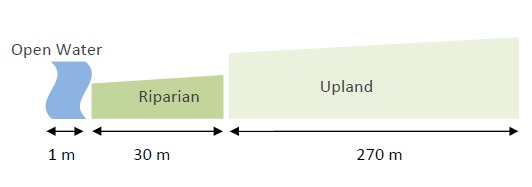
In accordance with the definition provided in the Conservation Blueprint, we consider stream systems to include 300 metres of riparian/upland area on either side of the stream. In order to differentiate between different restoration activities, stream systems are divided into three spatial categories:
- Open Waters – the width of the stream bed. We account for three categories of streams: headwaters (1 m stream width), middle tributaries (5 m stream width), and main stems (10 m stream width).
- Riparian – the area that extends to 30 m inland from either side of stream wetted edge.
- Upland 5 - the area that extends to 270 m inland beyond the end of the riparian area.
The diagram in Exhibit 2 presents an example of the three spatial categories using the headwater stream system width (1 m). The 300 m of riparian and uplands areas are present on both sides of the stream.
Exhibit 2 Spatial Diagram of Stream System Categories
1.3.3 Geographical Location
A preliminary analysis covered several Proposed Action Sites identified for the province of Ontario in the Conservation Strategy. The selected action sites (as identified in the Conservation Strategy) are: the Humber River – Toronto wetlands; the Credit River and Bronte-16 Mile Creeks; and, the Bay of Quinte. These sites link up fairly closely with the following “tertiary watersheds” in the Great Lakes Conservation Blueprint for Aquatic Biodiversity: Humber – Don Rivers (2HC)6; Credit River – 16 Mile Creek (2HB); and Prince Edward Bay (2HE). This analysis focuses on these three tertiary watersheds, as defined in the Conservation Blueprint.
1.3.4 Population Affected
The affected population includes those populations residing in each of the selected watersheds.
1.3.5 Time Frame for Analysis
Our timeframe for the analysis entails a period of 30 years which includes: 5 years for protective or restorative actions to take place; and, 25 years after protective or restorative actions have been completed.
1.3.6 Intervention Measures
A long list of ten potential intervention strategies was provided by the Steering Committee, in consultation with the Marbek team. Some of these strategies were proposed by the Great Lakes Regional Collaboration Strategy, the Great Lakes Habitat Initiative Final Report and Implementation Plan (USACE, 2008) and Ontario’s Biodiversity Strategy (2005).
For this report, we move from a long list of potential interventions to a short list used for cost/benefit analysis. In preparing the short-list of strategies, we consider the following additional criteria:
- There exists data to estimate or infer costs and benefits
- The impacts of interventions are presumably large
- The strategy is well defined
- It is feasible to complete the analysis within the timeframe and budget specified for this project
- There should not be overlaps with other theme areas of interest in this project
- Social marketing and behavioural strategies which cannot be easily quantified in a Cost- Benefit Analysis (CBA) are excluded.
A variety of methods are used to protect wetlands. These range from conserving land through transferring property ownership to voluntary private land stewardship practices. Each method yields different degrees of protection at different costs. Generally, higher investment costs afford the greatest level of protection. Successful habitat protection and restoration can:
- Achieve a sufficient, optimal size of natural cores and corridors
- Maintain high water quality and sustainable water balance
- Provide and protect habitat for wildlife and species-at-risk
- Conserve intact healthy natural areas for present and future generations.
For this study, we have selected two intervention strategies to include in our analysis:
- Land securement
- Restoration.
Land securement
For the purpose of this report, securement is defined as the protection of habitat by purchasing lands or acquiring the title to lands through donations. The more traditional means of securing land for conservation includes government purchases of land to create or expand provincial parks, conservation reserves, or protected areas. Land can also be purchased by private actors and non-governmental organizations. For example, five public and private groups have joined together this year (2010) to acquire 128 hectares of woods and wetlands near Kingsville, Ontario, which will expand the territory of the Cedar Creek Conservation Area. Land can also be purchased through donations. The Bruce Trail Conservancy is a charitable organization committed to protecting habitat along the Niagara Escarpment. Through donations, the Bruce Trail Conservancy has acquired several hundred acres of property that has served to secure continuous land corridors and thus protect important ecosystems and wildlife habitat.
Restoration
Land restoration is also known as land reclamation or rehabilitation, and it entails restoring a habitat that has been previously degraded to a more natural state, thus improving habitat/ecosystem functions and values. Our meaning of restoration leans more on the definition of rehabilitation whereby natural functions and processes that were disturbed are rehabilitated but the ecosystem itself will not necessarily be recovered to pre-disturbance conditions (Nolan, 2004). As an example of the variety and range of types of restoration activities, wetland restoration plans are extremely site specific and can employ various techniques. There are many variables to consider to ensure that wetland functions are restored and that restoration targets are achieved. Factors that affect wetland restoration design include size, position, proximity to other wetlands, forests, water bodies, or urban areas, local hydrology, depth to the water table, underlying sediment, vegetation, etc.. Similar factors contribute to the diversity of stream restoration activities. Wetland restoration measures include re-establishing water flows and/or water levels, re-establishing certain vegetation seedbanks and plant diversity, chemically or physically removing contaminants, and eliminating future source contamination (Environment Canada, 2010).
Other interventions (not included in our analysis)
Other interventions include conservation easements or agreements, land leases, or other informal stewardship agreements. A conservation easement is a voluntary, legal agreement between a landowner and a government agency (municipality, county, state, federal) or a qualified conservation group (sometimes called a land trust) that permanently restricts or prevents certain types of land uses, in order to protect its conservation value. Unlike land purchases, that require the landowner to sell or donate their property to a conservation organization, conservation easements allow private landowners to remain proprietor and continue to manage and use their land. Protection is achieved through unique terms of agreement for each easement. Common restrictions include the right to subdivide the property, to remove certain native vegetation species, and/or to build on the land (Ducks Unlimited Canada, 2010; Nature Conservancy Canada, 2010).
Land can also be protected through enhanced public policy and restrictive by-laws. For instance, zoning by-laws prevents building on significant wetlands, riparian by-laws require private owners to maintain riparian buffers within a minimal distance from streams or lakes, and recreational boating by-laws prohibit motor nautical vehicles from operating on certain sensitive water bodies.
These other interventions are more difficult to cost than land purchases or restoration because costs are extremely variable (in the case of land agreements) or they involve indirect costs (such as the opportunity costs related to by-law requirements). Furthermore, the benefits derived from these measures are difficult to estimate because the level of protection achieved is uncertain and dependent on compliance. Due to information and time limitations, the “Other Interventions” mentioned here are not included in the analysis for this report.
1.4 Overview of this Report
The remainder of this report is organized as follows:
- Section 2 Approach and Methodology
- Section 3 Analysis – Lake Ontario Watersheds
- Section 4 Results
- Section 5 Summary.
2.0 Approach and Methodology
This section provides background on total economic valuation (TEV), the framework that is used to categorize the different benefits. The approach and methodology is then divided into the different components of the analysis: cost-benefit analysis; and, uncertainty analysis. The economic impact analysis methodology and results are provided under separate cover.
2.1 TEV Framework
Habitats provide a wide array of benefits to society. Valuing these benefits is a challenge. The economic valuation method relates all the benefits to human welfare measures. The economic valuation method was chosen over alternative approaches because it allows for a robust measurement and comparison of values and presents these values in terms that people are familiar with. 7 Economic valuation is based on the notion of individual preferences, or what people want. The economic value of a good or service is the marginal willingness to trade that good or service for another.
While some goods and services have market values, many goods and services are not normally traded in a market. Therefore, nonmarket valuation techniques and methods are required to value these benefits to society. There are two main economic valuation methods of nonmarket goods and services: stated preference methods; and, revealed preference methods. Stated preference methods can estimate the TEV (use and non-use values) of nonmarket goods and services by using surveys to directly ask individuals what they would be willing to pay for changes in the quantity and/or quality of nonmarket goods and services. An example of this type of method is the contingent valuation method.
Revealed preference methods estimate the use-value of nonmarket goods and services by measuring relevant market behaviour. For example, the hedonic price method can be used to monetize various aesthetic and amenity values. This econometric approach involves gathering market data on property transactions and controlling for all the other features of a property (lot size, number of bedrooms, garage, etc.) except for the environmental amenity (proximity to lake, size of wetland, etc.) that is being valued. In this way, the value of the environmental amenity can be inferred from the revealed actions of individuals.
Both of these nonmarket valuation methods attempt to estimate the economic value of the various goods or services. The Willingness-to-Pay (WTP) metric is a measure of the maximum amount that individuals are willing to exchange for a good or service. The WTP for a good or service is therefore assumed to be the marginal level of human welfare that is derived from this good or service. In addition, it is assumed that societal values are simply the aggregation of individual values.
The type of benefits that the habitats provide can be categorized using the total economic valuation (TEV) framework. The appeal of using the TEV framework is that it is both logical and comprehensive. The logical nature of the framework comes from its foundations in microeconomic theory and emphasis on marginal values while the comprehensiveness stems from its ability to include all aspects of the habitat’s value. In addition, because this is the approach taken by economists in valuing environmental goods and services, the relevant literature can be consistently analyzed using this TEV framework. This framework considers that the benefits provided by habitats are linked to direct-use values, indirect use values(specifically, ecosystem services), option values, and non-use values. Exhibit 3 illustrates the type of values associated with the habitats within the TEV framework.
Exhibit 3 Total Economic Value of Natural Resources
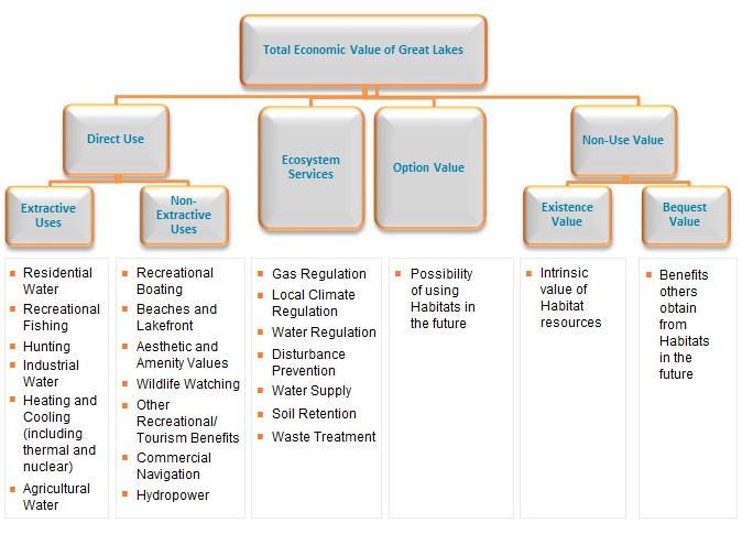
Direct use values reflect the direct use of the resource, like fish, water and space for recreation, and water use by agricultural and industrial/commercial firms (Tietenberg, 2006). Indirect use values include ways in which the lakes benefit communities by providing services such as waste assimilation and flood control. These indirect use categories can also be thought ecosystem of as services. 8
Option value refers to the option of using specific aspects of habitat in the future even if they are not being used today. Non-use values include existence and bequest values. Existence value recognizes that some Ontarians may be prepared to pay something for the protection and restoration of habitats, even if they do not currently use the watershed for recreation, fishing or any other activity. Bequest value recognizes that decisions regarding the watershed should also take into account the value of leaving them undamaged for future generations.
In addition to valuing these benefits, the value estimates need to be presented in a common metric so that benefit values may be compared to costs. In this analysis, dollars are used as the common numeraire so that values across goods and services can be easily compared. 9
Using these concepts, the TEV of the habitats can be presented using a common method (economic valuation) and metric (dollars).
Many of the values that can be attributed to natural watersheds are often ignored in private valuations and even in the evaluation of public projects. Historically, the focus of governments has been on the far left branch of Exhibit 3, namely on consumptive, direct use values, for which market values are often readily available. In this study we attempt to gather information on the other categories of values in addition to direct-use values to facilitate a more robust economic assessment.
2.2 Cost-Benefit Analysis Approach
2.2.1 Overview of Approach
Our cost-benefit analysis approach draws upon the principles and guidelines provided by the US Environmental Protection Agency,10 the World Bank,11 the Green Book of the UK,12 and the Canadian Cost-Benefit Analysis Guide for Regulatory Proposals.
For this study, the cost-benefit analysis consists of 10 tasks, which can be divided into four main phases.
- Phase I - Assess Background Study Boundary Data
- Task 1: Analyze habitat data and identify conservation goals for each watershed
- Task 2: Develop intervention strategy boundaries
- Task 3: Determine the portfolio of habitat interventions for each watershed
- Phase II - Value Costs of Habitat Interventions
- Task 4: Assess costs of interventions per unit area for each habitat type
- Task 5: Determine total costs of habitat intervention portfolios for each watershed
- Phase III - Value Benefits of Habitat Interventions
- Task 6: Link intervention strategies with benefits
- Task 7: Assess monetary value of benefits
- Task 8: Determine total monetary value of habitat intervention portfolios for each watershed
- Task 9: Describe intangible benefits
- Phase IV - Compare Costs and Benefits
- Task 10: Weigh benefits against costs.
2.2.2 Phase I – Assess Background Study Boundary Data
The Conservation Blueprint was consulted to select three watersheds in the Lake Ontario region that coincided with priority action sites identified in the Binational Biodiversity Conservation Strategy for Lake Ontario. The three watersheds empty into Lake Ontario and are identified as having a shortage of conserved habitat area.
Although this analysis is focused on the three selected watersheds, the approach used for cost- benefit analysis can be applied to any watershed, given that the appropriate input data is available. The results of this analysis will provide some indication of the expected magnitudes of costs and benefits in other watersheds, depending on certain comparable features such as demographics and land cover distribution.
Habitat data from the Conservation Blueprint for each habitat type (as listed in Exhibit 1) in each of the three target watershed groups were assessed to determine the additional area (in ha) needed to be conserved over and above the area currently conserved (identified as “all conservation lands” in the Conservation Blueprint) to meet the Conservation Blueprint goals for each watershed. According to the Conservation Blueprint, all conservation lands includes parks and protected areas and additional designated natural heritage areas (i.e., provincially significant life science Areas of Natural and Scientific Interest, Conservation Authority lands, provincially significant wetlands and Nature Conservancy of Canada lands). 13
Following the identification of conservation goals by habitat type for each watershed, a portfolio of habitat interventions was determined. The portfolio of intervention strategies is divided by land that should undergo: 1) securement only; and, 2) securement and active restoration.
Initially, the portfolio of intervention strategies was allocated to each habitat and watershed based on information from readily available documents, including the Biodiversity Conservation Strategy for Lake Ontario, the Great Lakes Conservation Blueprint for Aquatic Biodiversity, and watershed management plans. The intervention allocation for each habitat at a percentage level was then discussed with individual Conservation Authorities within each watershed to determine if the allocation is appropriate, based on their expertise and in-depth knowledge of their respective areas. The list of Conservation Authorities (including contact names) that were approached for information is found in Appendix F.
2.2.3 Phase II – Value Costs of Habitat Interventions
This section presents the methodology for costing our two intervention strategies: land securement and land restoration.
The main steps for costing the intervention strategies are:
- Identify costs of land securement for each watershed
- Develop a unit cost of restoration per hectare for each habitat type; and finally,
- Calculate an aggregate cost per hectare for each identified watershed using the selected portfolio of intervention strategies for each habitat type.
It is important to note that “restoration” will necessarily incur both the cost of active restoration and the cost of land value. In reality, land to be conserved may not actually need to be purchased because it may already be publicly owned, or private owners may incur the costs (for example, through donation of land or stewardship agreements). However, the purchase price is the opportunity cost to society of using the land as habitat compared to alternative uses (e.g., residential, commercial, industrial, etc.). Therefore, costs of interventions reflect all land that needs to be protected (thus implicitly purchased), and what percentage of this land should undergo active restoration (additional cost) versus being left as natural cover (regenerate growth). In other words, in this analysis land securement requires only the land purchase price, while active restoration requires both the land purchase price and the cost of restoration.
Land Securement
The cost to society of setting land aside for habitat is the value of the land in its next best alternative use. To estimate the value of the land in its next best alternative use, we use a hedonic price model based on market data of recent land purchases in the relevant watersheds (Sverrisson, 2008) and information from the 2006 Census of Agriculture. Therefore, land securement costs represent the purchase price for land in each watershed.
Restoration
Restoration costs were initially compiled from the literature, including Canadian cost data from the International Lake Ontario-St. Lawrence River Study Board (2006) for wetland restoration projects and USACE (2008) for stream systems restoration projects. These costs were compared against the cost estimates provided by individual Conservation Authorities. The rough estimates of project level costs or aggregate cost data for the types of projects that are commonly carried out in each jurisdiction were used to verify the cost data from the literature. Therefore, the costs are based on past experience with real restoration projects.
2.2.4 Phase III – Value Benefits of Habitat Interventions
This section presents the methodologies for valuing the benefits associated with the implementation of the Conservation Blueprint. Conceptually, we are estimating the economic benefits to Ontarians of protecting certain areas of wetlands, streams and riparian habitats (up to 300 metres on either side) in three tertiary watersheds. To estimate the value of converting these areas to protected habitat, we need to make an assumption about the alternative or counterfactual characteristics of these areas (i.e. if they remained unprotected). In this analysis it is assumed that in the absence of protection, the land will be developed and the habitats will be damaged and degraded. Therefore, the benefits are compared to a scenario where development of the land is complete. The exact nature of the development is not important, but we assume that full development of habitats results in zero ecosystem services from the land for society. 14 This is an important assumption because it generates a baseline that we can use to assess costs and benefits.
Background on Methodology
We do not conduct primary valuation estimation in this analysis, but rather we use benefit transfer as the valuation technique. Benefit transfer approaches are increasingly used because of time and resource constraints that limit the appropriateness of conducting primary valuation studies. Benefit transfer is the adaptation and use of economic information derived from existing literature to assign a monetary value to a specific site with similar resource and policy conditions. Typically, where the data was originally drawn from is considered the “study” site, and where the benefits are being transferred to is considered the “policy” site.
Benefit transfer is not a single approach, but rather refers to a collection of methods. The two main approaches 15 to transferring values from the study site to the policy site are:
- Unit Value transfer
- Single point estimate transfer
- Average value transfer
- Benefit Function transfer
- Demand or benefit function
- Meta-analysis.
Unit value transfer a single point estimate from one study site or average estimates from several study sites and applies these values to the policy site. Unit value transfer estimates the value of an environmental good or service at the policy site by multiplying the quantity of that good or service at the policy site by the mean unit value estimated at the study site. Unit values are presented as values per individual or household or values per unit of area. Adjustments to income or price levels are often made to account for differences between the policy and study sites. The main advantage of using unit value transfer is that it is simple and easy to understand. The main limitation of using unit value transfer is that it requires that the study site is similar to the policy site in content and context.
Benefit function transfer encompasses the transfer of a benefit or demand function from a study, or a meta-analysis function derived from several studies. A meta-analysis refers to a regression analysis which statistically summarizes the relationship between benefit measures and quantifiable characteristics of studies. The two main advantages of using a meta-analysis as a benefit transfer method are that it utilizes information from a large number of studies and the independent variables can be set at levels that are specific to the policy site. This second advantage allows, to some degree, the differences to be accounted for between the study site and the policy site. The main limitations of using a meta-analysis are that they are only as good as the quality of the underlying original valuation studies and the content and context of past studies need to be similar enough to be able to be combined and statistically analyzed.
Methodology
In this analysis, we employ both the unit value transfer and the benefit function transfer methods. Exhibit 4 summarizes the valuation method that will be used for the different habitat types.
| Aquatic Ecosystem | Habitat Boundaries | Valuation Method |
|---|---|---|
| Coastal | Shoreline (to Great Lakes) | Qualitative Discussion (data limitations) |
| Coastal | Open shoreline wetlands | Meta-Analysis |
| Coastal | Semi-protected wetlands (estuaries) | Meta-Analysis |
| Stream | Stream Systems | Unit Value Transfer |
| Wetlands | All other wetlands (e.g., marsh, bog, fen, swamp) | Meta-Analysis |
As shown in Exhibit 4, we monetize the benefits associated with coastal and non-coastal wetlands by means of meta-analysis and stream systems through unit value transfer.
Wetlands
The approach to estimating the economic value of wetlands is based on the results of two meta-analyses (Ghermandi et al., 2009 and Brander et al., 2010). As noted above, meta-analysis utilizes information from a large number of studies to statistically summarize the relationship between benefit measures and quantifiable characteristics of the studies. Therefore, meta- analyses are able to estimate a single wetland value (in terms of WTP) for a set of input variables.
A basic summary of the two meta-analyses is provided in Exhibit 5. The full meta-analysis results for both of these studies are presented in Appendix D.
| Ghermandi et al. 2009 | Brander et al. 2010 | |
|---|---|---|
| Geographic Coverage | The whole world | Temperate climate zone wetlands (mainly US and Europe) |
| Wetland types | Estuarine | Inland marshes |
| Wetland types | Marine | Peat bogs |
| Wetland types | Riverine | Salt marshes |
| Wetland types | Palustrine | Intertidal mudflats |
| Wetland types | Lacustrine | |
| Wetland types | Constructed | |
| Wetland types | Flood control and storm buffering | Flood control and storm buffering |
| Wetland types | Surface and groundwater supply | Surface and groundwater supply |
| Wetland types | Water quality improvement | Water quality improvement |
| Wetland types | Commercial fishing and hunting | Commercial fishing and hunting |
| Wetland types | Recreational hunting | Recreational hunting |
| Wetland types | Recreational fishing | Recreational fishing |
| Wetland types | Harvesting of natural materials | Harvesting of natural materials |
| Wetland types | Fuel wood | Fuel wood |
| Wetland types | Non-consumptive recreation | Non-consumptive recreation |
| Wetland types | Amenity and aesthetics | Amenity and aesthetics |
| Wetland types | Biodiversity | Biodiversity |
| Human pressure | Low pressure | N/A |
| Human pressure | Medium-low human pressure | N/A |
| Human pressure | Medium-high human pressure | N/A |
| Human pressure | High human pressure | N/A |
| Number of Observations | 418 | 264 |
As shown in Exhibit 5, both Ghermandi and Brander consider the same bundle of wetland services. 16 In addition, there are no valuation studies included in the meta-analysis for several categories of wetland services. We supplement the results of the meta-analysis by specific values for the regulation of greenhouse gases by wetlands from Troy and Bagstad (2009).
The specific steps for estimating the value of wetlands in our analysis are:
- Determine the variable values in the regression equation for each watershed. The meta-analyses of Ghermandi et al. (2009) and Brander et al. (2010) both include variables on real GDP per capita, population within 50 km, and wetland abundance within 50 km. 17 Besides large and small marshes, the Conservation Blueprint does not provide explicit information on the size of wetlands that should be protected. Therefore, we use 500 hectares as the average size of the large wetland category and 50 hectares as the average size of all the other wetlands. 18 In addition, Ghermandi et al. (2009) include variables on ‘human pressure’ and whether the wetland was constructed or not.
- Use the results of Phase I and the meta-regression function to estimate the per hectare annual value for each wetland in the watershed.
- Supplement the regression results for other wetland services not explicitly included in the meta-analysis (i.e. regulation of greenhouse gases).
- Multiply the per hectare site specific wetland values by the area of each wetland.
- Aggregate the results on a watershed level to determine the total economic benefits associated with fulfilling the Conservation Blueprint objectives for wetland protection.
The advantage of using this approach is that it explicitly incorporates variables on wetland size, real GDP per capita, neighbouring population levels and wetland abundance. All four of these factors have been found to influence the value of a wetland.
All previous valuations of wetlands in Canada that have used the benefit transfer approach have been conducted using variations of the unit transfer method. The meta-analyses used in this analysis represent the frontiers of environmental valuation literature. The results of the meta-analysis are compared to previous estimates of the economic values of wetlands. A summary of the other relevant wetland valuation studies is presented in Appendix C (Exhibit 46).
Stream Systems
The Conservation Blueprint considers stream systems to include 300 metres of riparian areas on either side of the stream. This area is much larger than the definition of riparian areas considered in the economic valuation studies by Troy and Bagstad (2009) (30 metres) and Kennedy and Wilson (2009) (15 metres). Ontario-specific results of Troy and Bagstad (2009) and Kennedy and Wilson (2009), both of which are themselves based on benefit transfer from a wide range of studies, are presented in Appendix C (Exhibit 47). Loomis et al. (2000) and Holmes et al. (2004) provide WTP measures based on original contingent valuation studies for a suite of intervention strategies related to restoring riparian areas and ensuring ecological integrity in Colorado and North Carolina respectively. The relevant study characteristics for Loomis et al. (2000) and Holmes et al. (2004) are summarized in Appendix C (Exhibit 48).
The approach to estimating the economic value of protecting stream and riparian habitat is to use the unit transfer method from a combination of the Troy and Bagstad (2009) report and the Loomis et al. (2000) study because we consider these to be the most rigorous of the studies and because they are the closest fit to the intervention strategies being evaluated here. We adjust the benefit values in both studies as explained below to conform as closely as possible to the characteristics of the watersheds being considered.
Two valuation methodologies are adopted and the results are compared to test the robustness of our approach. To illustrate the two methodologies, we use Credit River – 16 Mile Creek watershed as an example and focus on main stem waters only.
Illustration of Stream Systems Valuation Method 1
It is estimated that the area to be added to protection that borders and includes main stem rivers is 4,571.4 hectares. To perform a benefit transfer analysis using the Troy and Bagstad (2009) study, we must break this total area down into the area that is strictly open water, the area that is within 30 metres of open water, and the remaining land. We do this by assuming an average width for the open water of the main stem and then perform the necessary calculations. The benefit transfer analysis is then conducted using the per-hectare values in Troy and Bagstad (2009) as follows:
- The Troy and Bagstad (2009) values per hectare of open water depend on whether it is urban ($237,013) or non-urban ($55,699) open water. Therefore, through consultation with Conservation Authorities, we estimated the percentage of stream systems in urban versus non-urban areas. This same percentage was then applied to the areas to be protected to determine the urban versus non-urban proportions. The weighted average per-hectare value of open water (weighted by the proportion of urban versus non-urban area) is then multiplied by the number of hectares of open main stem water.
- For the riparian buffer strip 30 metres on either side of the open water, we multiply the Troy and Bagstad (2009) values for “Forest adjacent to stream” ($4,564/ha) by the number of hectares of riparian land.
- For the remainder of the land area either side of the river, we multiply the Troy and Bagstad (2009) value for “Forest non-urban” ($4,455/ha) by the remaining area.
Method 1 was applied to the Headwaters and Middle Tributaries areas as well. A total value was then calculated for the increased area to be added to habitat protection.
Exhibit 6 provides a summary of which benefits are included in the Troy and Bagstad (2009) values. As shown, water quality improvements are the ecosystem service with the highest value for forests adjacent to streams and non-urban/suburban open water. In the case of urban/suburban open water, recreation benefits have the highest ecosystem benefits.
| Source | Location | Habitat Type | Benefits Included in the Analysis | Habitat Value per Hectare |
|---|---|---|---|---|
| Troy and Bagstad (2009) | Southern Ontario | Forest adjacent to a stream | Recreation | $560 |
| Troy and Bagstad (2009) | Southern Ontario | Forest adjacent to a stream | Habitat refugium and Biodiversity | $133 |
| Troy and Bagstad (2009) | Southern Ontario | Forest adjacent to a stream | Atmospheric Regulation | $995 |
| Troy and Bagstad (2009) | Southern Ontario | Forest adjacent to a stream | Soil Retention/Erosion Control | $781 |
| Troy and Bagstad (2009) | Southern Ontario | Forest adjacent to a stream | Water Quality/nutrient & waste regulation | $614 |
| Troy and Bagstad (2009) | Southern Ontario | Forest adjacent to a stream | Water Supply/Regulation | $1,323 |
| Troy and Bagstad (2009) | Southern Ontario | Forest adjacent to a stream | Disturbance Avoidance | $148 |
| Troy and Bagstad (2009) | Southern Ontario | Forest adjacent to a stream | Total | $4,564 |
| Troy and Bagstad (2009) | Southern Ontario | River (open water) | Recreation | $8,678 |
| Troy and Bagstad (2009) | Southern Ontario | River (open water) | Other Cultural | $25 |
| Troy and Bagstad (2009) | Southern Ontario | River (open water) | Habitat refugium and Biodiversity | $10 |
| Troy and Bagstad (2009) | Southern Ontario | River (open water) | Water Quality/nutrient & waste regulation | $33,996 |
| Troy and Bagstad (2009) | Southern Ontario | River (open water) | Water Supply/Regulation | $12,991 |
| Troy and Bagstad (2009) | Southern Ontario | River (open water) | Total | $55,699 |
| Troy and Bagstad (2009) | Southern Ontario | Urban/suburban river (open water) | Recreation | $173,148 |
| Troy and Bagstad (2009) | Southern Ontario | Urban/suburban river (open water) | Aesthetic and Amenity | $243 |
| Troy and Bagstad (2009) | Southern Ontario | Urban/suburban river (open water) | Water Quality/nutrient & waste regulation | $45,889 |
| Troy and Bagstad (2009) | Southern Ontario | Urban/suburban river (open water) | Water Supply/Regulation | $17,737 |
| Troy and Bagstad (2009) | Southern Ontario | Urban/suburban river (open water) | Total | $237,013 |
Illustration of Stream Systems Valuation Method 2
We use both the Loomis et al (2000) and the Troy and Bagstad (2009) studies for benefit transfer in method 2. The Loomis et al (2000) study estimated the value of restoring ecosystem services in an impaired river basin in the South Platte River near Denver Colorado to be $252 per household for households living within the counties through which a 45 mile stretch of the river flows. Loomis et al. (2000) explicitly consider five ecosystem services:
- dilution of wastewater;
- natural purification of water;
- erosion control;
- habitat for fish and wildlife; and,
- recreation.
After converting to Canadian currency and adjusting for inflation, this value becomes about $375. We allow for a further adjustment to this value to transfer it to an Ontario context. Specifically, an adjustment factor is applied in recognition of the Johnston and Thomassin (2010) finding that Canadians’ WTP estimates are lower than those in the US. Based on the results of their study, we set the adjustment factor at 0.16 (meaning only 16% of the Loomis value is used for benefits transfer). 19 Accordingly, we multiply $375 by the adjustment value of 0.16 and then by the number of households that live within a 50 km radius of the watershed. This gives an estimate of the total value of the five improved ecosystem functions included in the Loomis study in the open water and the 30 meter riparian buffer strip.
To this aggregate value, we add the value of “atmospheric regulation” from Troy and Bagstad (2009) (as this ecosystem service was not considered in the Loomis et al study) in that part of the 30 metre riparian strip that is currently not under natural cover. For the remaining adjacent land not under natural cover out to 300 metres on either side of the water, we use the value of all ecosystem services considered in Troy and Bagstad (2009) for “Forest: non-urban” except those associated with improvements in water quality and nutrient and waste regulation because Loomis et al (2009) already include these values in their surveys, and we assume these values extend out to the full 300 metres on either side of the open water.
Note finally that one of the values we were not able to estimate is the downstream benefit of protecting and/or restoring upstream habitat. The reason is that we have no information about the expected improvement in downstream water quality that results from the restoration of upstream habitat.
2.2.5 Phase IV – Compare Costs and Benefits
In this analysis, we are comparing the costs of habitat restoration and protection interventions that occur over five years with benefits that accrue over multiple years. Therefore, we need to make assumptions about the timing of benefits and choose a discount rate which will allow us to aggregate the stream of costs and benefits into a single present value metric. In this analysis, we make the simplifying assumption that benefits do not begin to accrue to society until after all of the habitat types have been purchased or restored. Thus, society starts receiving the benefits of habitat restoration and protection in year 6. On the one hand, this assumption will tend to underestimate the economic benefits that would be realized in a relatively short time frame (i.e. water quality after a stream restoration project). On the other hand, this assumption overestimates the economic benefits that may take a relatively longer time frame to be realized (i.e. carbon sequestration of newly restored riparian areas).
Discount Rate
The choice of a Social Discount Rate (SDR) is an important and controversial policy decision in cost benefit analysis. For our study, we considered the two main approaches that exist for calculating the discount rate:
- The social opportunity cost rate of capital
- The social time preference rate.
The social opportunity cost rate of capital is usually identified as the real rate of return earned on a marginal project in the private sector. The social time preference rate is the rate at which society is willing to trade off between present and future consumption. This rate takes into account factors other than the economic opportunity cost of funds and is often used for circumstances where environmental goods and services are substantial.
Current “interim” guidelines from the Treasury Board Secretariat (TBS) use a weighted social opportunity cost rate of capital approach to recommend a SDR of 8% with sensitivity rates of 3% and 10%. However, this choice has been severely criticized for not reflecting relevant theoretical and empirical literature.
There is now widespread agreement that the most appropriate method for calculating the SDR is through the use of an optimal growth rate model. Using this method, the SDR depends on three primary variables and is formulated as:
SDR = d + e×g
The first term, d, is the utility discount rate (“pure preference for utility in the present over the future”, Boardman et al., 2009). The latter product term is composed of e, the elasticity of marginal utility with respect to consumption (i.e. the absolute value of the rate at which the marginal value of consumption decreases as per-capita consumption increases) and g, the growth in per-capita consumption.
Using this approach, Boardman et al. (2009) proposes that Canada should use a SDR of 3.5% with sensitivity rates of 2% and 5% for intragenerational projects. This SDR is a real, before- inflation rate. To arrive at a central SDR estimate for Canada of 3.5%, Boardman et al. (2009) use values of d = 1, e = 1.5 and g = 1.7.
The research and policy trend in other countries also supports using a relatively low social discount rate. In the US, Moore et al. (2004) propose a SDR of 3.5% in many circumstances. The United Kingdom government has recently lowered their recommended SDR from 6% to 3.5% (HM Treasury (2003)). Finally, in France, a reduction in the SDR from 8% to 4% has recently been recommended by a group of experts commissioned by the ministry of Finance (Lebegue et al., 2005).
For the purpose of this economic analysis, we use a SDR of 3.5% with sensitivity rates of 2% and 5%. We feel this SDR is appropriate because it reflects both the specific circumstances of the economic analysis and the recent theoretical and empirical literature.
2.3 Uncertainty Analysis Approach
A risk-based analysis was conducted to ensure that the final results (net present value) reflect the uncertainty in key input variables. To account for the inherent uncertainties involved, Monte Carlo simulations using @Risk Software were performed. 20 This approach integrates uncertainty into the analysis as opposed to relying on ex post sensitivity analysis to test the robustness of the results. This approach allows us to describe a distribution of possible economic benefits rather than specific point estimates. This analysis is important to test the robustness of the results for changes in various variables. In addition, the range of outcomes that the net benefit falls within can then be identified, and the risk of a negative outcome (costs > benefits) better understood.
Uncertainty is factored into the analysis through the definition of uncertainty ranges around key variables. In the cases where we have a range of values, we use these as our low and high values, with the average as the most likely. In the cases where we have single point estimates, we use this as the most likely and add/subtract 25% to arrive at our high/low estimates. Thus, uncertainty is factored into our analysis by considering a range of possible values.
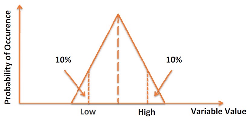
To keep the analytics of @Risk simple, we use the RiskTrigen function. 21 This triangular distribution function specifies three points: one at the most likely, one at the specified bottom percentile and one at the specified top percentile. The percentile values give the percentage of the total area under the triangle that falls to the left of the entered point. Using this distribution, we attach small probabilities that the costs and benefits will fall beyond our high or low estimates. More information regarding how the values derived in this report are used in the @Risk software is provided in Section 3.2.
Exhibit 7 presents a graphical representation of the probability distribution of the RiskTrigen function. The variable values are distributed along the X-axis and the probability of occurrence is represented on the Y-axis. As shown, the central dashed line has the highest probability of occurrence and the probability of occurrence decreases as the variable values move further away from this central estimate.
Exhibit 7 The RiskTrigen Function in @Risk
2.4 Economic Impact Analysis Approach
Completed under separate cover.
3.0 Analysis – Lake Ontario Watersheds
3.1 Cost-Benefit Analysis
This section presents the analysis for estimating the costs and benefits in the three selected watersheds. The sub-sections reflect the four phases discussed in Section 2.2.
3.1.1 Phase I – Background Study Boundary Data
Exhibit 8, Exhibit 9, and Exhibit 10 present the additional area required for each habitat system in each watershed to reach the Conservation Blueprint goals. Additional area to conserve refers to the additional area (beyond the areas already protected in existing conservation lands) requiring protection to reach the Conservation Blueprint goals. This analysis assumes that all conservation lands are in natural cover.
The data is divided as follows:
- Total additional area (Additional area (ha) to conserve)
- Additional area that needs to be conserved that is already under natural cover (the quality of which is unknown) (Area (ha) needed already in NC)
- Additional area that needs to be conserved that is not in natural cover (Area (ha) needed not in NC)
This division of area is necessary in order to distinguish between areas that can be protected and left to regenerate on their own, and areas that require active restoration prior to protection (which would include all areas not under natural cover).
| Habitat System | Total area (ha) in WS 2HB | Total area (ha) in all CL | Area (ha) in BP | Area (ha) in BP under NC | Additional area (ha) to conserve | NC not yet conserved | Area (ha) needed already in NC | Area (ha) needed not in NC |
|---|---|---|---|---|---|---|---|---|
| Shoreline | 76.8 | 4.9 | 51.0 | 51.0 | 46.06 | 46.1 | 46.1 | 0.0 |
| Headwaters | 154342.4 | 8217.1 | 16677.5 | 11666.1 | 8460.4 | 3449.1 | 3449.1 | 5011.4 |
| Middle Tributaries | 46041.3 | 3673.4 | 19865.8 | 7965.1 | 16192.4 | 4291.7 | 4291.7 | 11900.7 |
| Main Stem | 4603.6 | 31.3 | 4602.8 | 443.6 | 4571.4 | 412.3 | 412.3 | 4159.2 |
| Large Wetlands | 291.1 | 287.6 | 291.1 | 291.1 | 3.5 | 3.5 | 3.5 | 0.0 |
| Other Wetlands | 14195.0 | 11964.6 | 12053.2 | 12053.2 | 88.6 | 88.6 | 88.6 | 0.0 |
| Other | 8974.3 | 49.4 | 1930.1 | 155.8 | 1880.7 | 106.4 | 106.4 | 1774.3 |
| Habitat System | Total area (ha) in WS 2HC | Total area (ha) in all CL | Area (ha) in BP | Area (ha) in BP under NC | Additional area (ha) to conserve | NC not yet conserved | Area (ha) needed already in NC | Area (ha) needed not in NC |
|---|---|---|---|---|---|---|---|---|
| Shoreline | 228.1 | 86.3 | 136.2 | 136.2 | 49.9 | 49.9 | 49.9 | 0.0 |
| Open Shoreline Wetlands | 8.3 | 4.9 | 7.4 | 7.4 | 2.6 | 2.6 | 2.6 | 0.0 |
| Semi-Protected Wetlands | 0.4 | 0.0 | 0.5 | 0.5 | 0.5 | 0.5 | 0.5 | 0.0 |
| Headwaters | 174572.8 | 10566.6 | 20276.9 | 14652.7 | 9710.3 | 4086.1 | 4086.1 | 5624.2 |
| Middle Tributaries | 50685.7 | 4072.6 | 8315.8 | 5693. | 4243.2 | 1620.4 | 1620.4 | 2622.8 |
| Main Stem | 15882.5 | 2829.0 | 11550.6 | 4149.5 | 8721.6 | 1320.5 | 1320.5 | 7401.1 |
| Other Wetlands | 3883.8 | 2998.9 | 3020.4 | 3020.6 | 21.5 | 21.6 | 21.5 | 0.0 |
| Other | 17069.4 | 520.5 | 5096.9 | 663.6 | 4576.4 | 143.1 | 143.1 | 4433.4 |
| Habitat System | Total area (ha) in WS 2HB | Total area (ha) in all CL | Area (ha) in BP | Area (ha) in BP under NC | Additional area (ha) to conserve | NC not yet conserved | Area (ha) needed already in NC | Area (ha) needed not in NC |
|---|---|---|---|---|---|---|---|---|
| Shoreline | 1282.9 | 141.3 | 176.6 | 176.6 | 35.3 | 35.3 | 35.3 | 0.0 |
| Headwaters | 76169.6 | 1210.7 | 13375.8 | 9027.3 | 12165.1 | 7816.6 | 7816.6 | 4348.6 |
| Main Stem | 160.3 | 20.4 | 47.9 | 47.9 | 27.5 | 27.5 | 27.5 | 0.0 |
| Large Wetlands | 2872.6 | 2644.8 | 2871.6 | 2871.6 | 226.8 | 226.8 | 226.8 | 0.0 |
| Other Wetlands | 12934.4 | 5287.4 | 6033.3 | 6033.2 | 745.9 | 745.8 | 745.8 | 0.1 |
| Other | 12604.4 | 923.0 | 1533.3 | 1473.8 | 610.3 | 550.8 | 550.8 | 59.6 |
As noted above, the additional area required for conservation was divided into land under natural cover and land not under natural cover. This division of area was necessary in order to distinguish between areas that can be protected and left to regenerate on their own, and areas that require active restoration prior to protection.
All land not in natural cover would need to be restored prior to protection. For example, a strip of cropland that directly borders a stream would have to be secured for protection as well as actively restored to natural cover (i.e., restore it to a natural riparian buffer). Land that currently exists under natural cover may either require restoration prior to protection or only protection, depending on the quality of the natural cover. For example, a wetland is considered 100% natural cover. However, depending on the condition of the wetland, it may need to be actively restored as well as secured for protection. If the wetland is in poor condition, active restoration would be required in addition to protection. If the wetland is still functional, it could be protected and left to regenerate on its own.
Following the identification of conservation goals by habitat type for each watershed, the next step was to determine a portfolio of habitat interventions. The portfolio of interventions is specific to each watershed and based on the two interventions in our analysis (restoration and protection (land securement)).
Exhibit 11, Exhibit 12, and Exhibit 13 present the percentage of land for the intervention strategies allocated to each habitat and watershed. The optimal mix between restoration and protection interventions needed to achieve the conservation goals were based initially on information from readily available documentation noted in Section 2.2.2 and then verified, or modified as needed, with the help of Conservation Authorities. We relied on the experience and depth of knowledge of the Conservation Authorities to estimate a reasonable level of active restoration versus natural cover that could be purchased/protected and left to regenerate on its own for each habitat. The list of questions submitted to the Conservation Authorities can be found in Appendix F.
| Habitat System | Additional area (ha) to conserve | Intervention * - Active Restoration | Intervention * - Purchase / Protection |
|---|---|---|---|
| Shoreline | 46.06 | 100% | 0% |
| Headwaters | 8460.4 | 80% | 20% |
| Middle Tributaries | 16192.4 | 80% | 20% |
| Main Stem | 4571.4 | 80% | 20% |
| Large Wetlands | 3.5 | 80% | 20% |
| Other Wetlands | 88.6 | 80% | 20% |
| Other | 1880.7 | 80% | 20% |
| Habitat System | Additional area (ha) to conserve | Intervention * - Active Restoration | Intervention * - Purchase / Protection |
|---|---|---|---|
| Shoreline | 49.9 | 100% | 0% |
| Open Shoreline Wetlands | 2.6 | 100% | 0% |
| Semi-Protected Wetlands | 0.5 | 100% | 0% |
| Headwaters | 9710.3 | 100% | 0% |
| Middle Tributaries | 4243.2 | 100% | 0% |
| Main Stem | 8721.6 | 100% | 0% |
| Other Wetlands | 21.5 | 100% | 0% |
| Other | 4576.4 | 100% | 0% |
| Habitat System | Additional area (ha) to conserve | Intervention * - Active Restoration | Intervention * - Purchase / Protection |
|---|---|---|---|
| Shoreline | 35.3 | 30% | 70% |
| Headwaters | 12165.1 | 40% | 60% |
| Main Stem | 27.5 | 40% | 60% |
| Large Wetlands | 226.8 | 40% | 60% |
| Other Wetlands | 745.9 | 40% | 60% |
| Other | 610.3 |
* Assumes that lands undergoing Restoration are also protected; and Purchase/Protection refers to the acquisition of land, which is left to regenerate on its own.
Coastal shoreline (to the Great Lakes) is included for qualitative discussion only. Intervention strategies for shoreline are not carried through in the cost benefit analysis due to data limitations.
3.1.2 Phase II – Costs
Using the approach outlined in Section 2.2.3, we estimate the cost of protecting wetlands and streams in the three selected watersheds, by use of our two selected intervention strategies.
Land Securement
To determine the opportunity cost of using the land in its next alternative use, we use two methods to derive a low and high estimate. The first method uses the hedonic study by Vyn (2007) (as summarized in Sverrisson, 2008). The second method uses Statistics Canada data on the value of agricultural land in each of the three watersheds. Using both methods, our aim is to derive location specific land securement costs for the three watersheds.
Vyn (2007) uses vacant land sale prices for 1,935 properties in the region around Toronto stretching from Lake Huron to Peterborough. Vyn’s (2007) data set includes land quality variables, neighbourhood and amenity variables and location variables. Because we do not have site specific data on potential land to be purchased in the watersheds, we cannot include land quality variables such as percentage of land with organic soil and number of crop heat units. Instead, we set all the land quality and neighbourhood and amenity variables in Vyn’s (2007) model to their mean values. 22 The county specific dummy variables allow the estimation of the cost of vacant land in specific counties. Therefore, we set the dummy variable for each respective county to the fraction of the watershed’s conservation goal (all other county specific variables are set to 0). However, in their analysis they do not include any counties that overlap with Prince Edward Bay. Therefore, because it is right beside the watershed, we use Northumberland county as a proxy for estimating land prices in Prince Edward Bay. The remaining two watersheds intersect with multiple counties. Credit River – 16 Mile Creek is located within Hamilton, Halton and Wellington counties while Toronto Area watersheds partly cover Peel and York counties. To account for this overlap between watersheds and counties, we determine the approximate percentage of the conservation goal areas for each watershed that fall into each county. For Credit River – 16 Mile Creek, we assume that Hamilton, Halton and Wellington counties constitute 20%, 40% and 40% of the conservation goal areas for the watershed, respectively. For Toronto Area, we assume that 50% of the conservation goal areas for the watershed are found within Peel county and 50% within York County. Appendix A presents Vyn’s (2007) land pricing model used in this analysis.
Using this model, we are able to estimate the cost to society of setting aside land for habitat protection. This results in a property purchase price per hectare of $35,732 for Credit River – 16 Mile, $89,656 for Toronto Area and $6,843 for Prince Edward Bay.
The second method uses the 2006 Census of Agriculture data on the total building and land value at the county level. These values can be divided by the number of hectares of agricultural land to determine the average value of farm land per hectare. Using the same assumptions of watershed overlap with counties, the average per hectare value of farmland is $22,918 for Credit River – 16 Mile, $41,268 for Toronto Area and $6,472 for Prince Edward Bay. These farmland values are less than half of the cost per hectare estimated using the hedonic price model for Credit River – 16 Mile and Toronto Area. Interestingly, the farmland value for Prince Edward Bay of $6,472 is very close to our estimated land value of $6,843. These two methods provide a low and a high estimate of the potential opportunity cost to society of purchasing land for habitat for protection. 23
To validate these cost estimates we also examined other sources of data. From 1996 to 2006, the Nature Conservancy of Canada and Ontario Parks has invested $21.9 million dollars to purchase 17,064 hectares of land in Ontario, for an average per hectare price of $1,286 (Sverrisson, 2008). This value is substantially lower than any of our cost estimates using the hedonic price model. More specific watershed data from the Nature Conservancy of Canada show that recent acquisitions in the Humber River watershed have averaged $33,699 per hectare. This is below our estimated value for this watershed of $89,656. By using the latter purchase price, we may be over-estimating costs, and we are ensuring a conservative and defensible cost-benefit analysis. However, the fact that NCC relies to a large extent on charitable donations, the lands it can afford may not represent the baseline costs for this comparison.
Exhibit 14 summarizes the costs of purchasing land for the three watersheds.
| Credit River – 16 Mile Creek - Low | Credit River – 16 Mile Creek - High | Toronto Area - Low | Toronto Area - High | Prince Edward Bay - Low | Prince Edward Bay - High | |
|---|---|---|---|---|---|---|
| Number of hectares | 29,093.5 | 29,093.5 | 22,505.4 | 22,505.4 | 13,144.6 | 13,144.6 |
| Cost per hectare | $22,918 | $35,732 | $41,268 | $89,656 | $4,993 | $8,321 |
| Total Cost of purchase | $666,777,551 | $1,039,564,070 | $928,744,191 | $2,017,738,355 | $67,456,711 | $112,427,852 |
Restoration: Wetlands
To estimate restoration costs for wetlands, we use Canadian cost data from the International Lake Ontario-St. Lawrence River Study Board (2006). The costs per hectare range from $3,240 to $1,368,121 and the average cost per hectare for these restoration projects is $57,802. This study reviews 60 wetland restoration projects administered by Environment Canada and U.S. Army Corps of Engineers. The Canadian projects are Great Lakes Sustainability Fund projects. The authors provide data on area restored, total and annualized project costs, and annual operating and maintenance costs. 24 The summary of costs for all Canadian projects included in this study is shown in Appendix B, Exhibit 40. The range of cost is quite large, reflecting the varying level of effort required for restoration projects. These projects can range from very simple measures such as planting of key vegetation species to major excavation works. Projects include establishment, re-establishment, rehabilitation, enhancement and protection of wetlands. We use the average costs per hectare of wetland restoration projects in our analysis.
We cross check our estimates with other costs from the literature and from personal communication with Conservation Authorities. For example, the Toronto and Region Conservation Authority has noted that the approximate upfront cost for swamp habitat restoration in their Conservation Authority area is $20,000 per hectare with ongoing maintenance costs of $6,000 for roughly 5 years (Lewis, 2010). These costs can be converted into a present value cost of approximately $47,090. 25 In addition, The Great Lakes Habitat Initiative Database reports an average cost per hectare for wetland restoration projects of $19,278. By using the wetland restoration cost of $57,802, we are ensuring we will not underestimate costs. Although this cost may potentially be an overestimate, a higher cost may account for the increased cost of operations in an urban setting such as the Rouge watershed. Furthermore use of a higher cost estimate results in a more conservative benefit-cost ratio.
Exhibit 15 presents the total average costs of restoration projects for each watershed, based on the number of hectares that need to be actively restored and the price of restoration projects per hectare. As shown, the project cost per hectare is the same across the three watersheds. We are unable to adjust these estimates for underlying wetland quality due to data limitations. 26
| Credit River - 16 Mile Creek | Toronto Area | Prince Edward Bay | |
|---|---|---|---|
| Number of hectares | 73.7 | 24.6 | 389.1 |
| Project Cost per hectare | $57,802 | $57,802 | $57,802 |
| Total Cost of Restoration Project | $4,257,152 | $1,419,773 | $22,488,051 |
Restoration: Streams
There are various sources of data on the cost of stream and riparian area restoration projects (Nolan, 2004; City of Toronto, 2003; Tejani et al., 2003; Hasset et al., 2005). However, this cost data is difficult to apply to our selected areas to be protected as it is most often reported as a cost per length of stream. Other unit cost measures are per width of stream, per project, or per restoration measure. For the purpose of consistency, we use values reported in the Great Lakes Habitat Initiative Final Report and Implementation Plan (USACE, 2008). This study collected data from nearly 200 restoration projects from federal, state, and NGO agencies, and compiled it into a project database. This inventory includes restoration projects for open and nearshore waters, riparian areas, upland area, and wetland areas. A summary of the data provided in this study is presented in Appendix B, Exhibit 40. As with wetland restoration costs, cost data from the literature was verified against estimates provided from individual Conservation Authorities.
Stream restoration costs are divided into three categories, as defined in Section 1.3.2:
- Open waters – Restoration activities for open waters include dredging sediments, restoring stream connectivity, creating islands or spawning areas, removing dams, and removing invasive species. These projects are expected to improve the habitat of several fish communities, benthic macroinvertebrates, as well as waterfowl and other birds (USACE, 2008). The average cost for these restoration projects is $121,992 per hectare (USACE, 2008). It is difficult to compare and validate costs among various data sources because these are reported under different unit costs: per project, per stream length, by stream width, per hectare, or per restoration measure. The Credit Valley Conservation Authority reported that the average cost per hectare for restoration projects (including stream, riparian, and wetland habitat) is approximately $24,248 (Hayes, 2010). By using an average cost of $121,992 per hectare, we are probably using a conservative estimate and ensuring that costs are not under-reported
- Riparian – Restoration activities for the 30 m of riparian area bordering streams include bank stabilization, riparian habitat installation, removal of invasive species, installation of lamprey or carp barriers, culvert replacement, re-meandering channelized streams and rivers, removal of concrete substrate lining, and reconnecting floodplains. These restoration projects are intended to ensure their connectivity to floodplains and restore natural flow and sediment regimes. Consequently, this is identified to improve the habitat of numerous aquatic species, birds and waterfowls, reptiles, and mammals. The average cost for these restoration projects is $20,031 per hectare (USACE, 2008).
- Upland – Restoration for the 270 m of land extending beyond the riparian area include toxic sediment removal or remediation, tree-planting, installing native plants as a way to stabilize upland areas and increase habitat diversity, and erosion control along ravines. This type of restoration work is intended to improve wildlife habitat, increase habitat diversity, provide erosion control, and to support the natural processes that provide supporting and regulating ecosystem services. The average cost for these restoration projects is $2,395 per hectare (USACE, 2008). The Credit Valley Conservation Authority reported that the average cost per hectare for forest/woodland Reforestation projects is approximately $2,900 (Hayes, 2010).
Once per hectare restoration and land securement costs are established, they are multiplied by the respective area of restoration and land securement needed for habitat protection in each watershed. Exhibit 16, Exhibit 17, and Exhibit 18 present the total average costs of three categories of stream system restoration projects for each watershed, based on the number of hectares that need to be actively restored and the price of restoration projects per hectare.
| Open Water | Riparian Area | Upland | |
|---|---|---|---|
| Number of hectares | 178.3 | 2,320.1 | 20,881.0 |
| Restoration Costs per hectare | $121,992 | $20,031 | $2,395 |
| Total Cost of Restoration | $21,747,853 | $46,474,546 | $50,011,093 |
| Open Water | Riparian Area | Upland | |
|---|---|---|---|
| Number of hectares | 194.2 | 2,248.1 | 20,232.8 |
| Restoration Costs per hectare | $121,992 | $20,031 | $2,395 |
| Total Cost of Restoration | $23,691,172 | $45,031,767 | $48,458,523 |
| Open Water | Riparian Area | Upland | |
|---|---|---|---|
| Number of hectares | 8.3 | 486.9 | 4,381.9 |
| Restoration Costs per hectare | $121,992 | $20,031 | $2,395 |
| Total Cost of Restoration | $1,009,721 | $9,752,716 | $10,494,863 |
3.1.3 Phase III – Benefits
Wetlands
Using the approach outlined in Section 2.2.4, we can estimate the value of wetlands in the watersheds. First, we need to collect various data points and determine variable values to insert into our regression equation. For our meta-analysis we need to determine:
- Which wetland services to include in the analysis,
- GDP per capita,
- Population and wetland abundance in a 50 km radius,
- Wetland sizes, and
- Degree of anthropogenic pressure.
We need to determine which of the 11 wetland services included in Brander et al. (2010) and Ghermandi et al. (2009) (as presented in Exhibit 5) do not apply for our study areas. The only wetland service that is inappropriate for our analysis is their “Fuel wood” variable because residents are not collecting fuel wood from wetlands in Ontario. This variable is not included in the analysis (we set the dummy variable to 0 in the regression). The remaining 10 wetland services are included in the valuation analysis.
To determine the GDP per capita we collect income information from the relevant census districts from the 2006 Census by Statistics Canada 27. We use income per capita as a close approximation to GDP per capita, as the latter does not exist at the district level. We adjust the income per capita to 2003 US dollars as required for the meta-analysis equations. 28
The two meta-analyses include population and wetland abundance within a 50 km radius of the wetland site. Therefore to ensure consistency with these studies, we also need to determine the population and wetland abundance in a 50km radius.
To determine the population in a 50km radius, we follow these steps:
- Collect population and land area (square km) data for the relevant census districts from the 2006 Census to determine the relevant population densities (people per square km).
- Multiply the population density by the area of a 50 km circle (7,854 km2) to determine the population in a 50 km radius.
To determine the wetland area in a 50 km radius, we follow similar steps:
- Using the total area of wetlands and total size of the relevant watershed from the Conservation Blueprint, determine the wetland density (hectares of wetlands in each square km of watershed). Of course, we need to include the wetlands that will be protected and restored in this calculation because wetland abundance impacts our benefit estimation.
- Multiply the wetland density by the area of a 50 km circle (7,854 km2) to determine the wetland area in a 50 km radius.
It is important to note that Prince Edward Bay is fronted by water on one side. Therefore, the approach used above is inappropriate for this watershed. Instead, to estimate relevant population densities, we simply sum the population numbers from the Prince Edward census division and the neighbouring Belleville census agglomeration. This method will result in a somewhat conservative estimate of the population in a 50 km radius. For wetland abundance, we adjust our wetland abundance measure downwards by a factor of two to account for the fact that roughly one half of our area within a 50 km radius is covered by water.
For wetland size, we assume that the average size of a wetland in the large wetland category (greater than 100 ha) is 500 hectares and the average size of a wetland in the other wetland category is 50 hectares. Of course, wetland sizes vary along a wide gradient from one hectare to well over 500 hectares. For our purposes, defining only two categories of wetland sizes is necessary in the absence of more refined data. 29
Finally, for the Ghermandi et al. (2010) meta-analysis, we need to determine the degree of anthropogenic pressure exerted on wetlands in our three watersheds. Ghermandi et al. (2010) consider three criteria to determine the state of human pressure. 30 These criteria rank from lowest level of human pressure (low human pressure) to the highest level of human pressure (high human pressure) with two intermediate states (medium-low and medium-high human pressure). We determine the percentage of wetlands in each watershed that fall into the four states of human pressure.
| Variable | Credit River- 16 Mile Creek | Toronto Area | Prince Edward Bay |
|---|---|---|---|
| GDP per capita ($2003 USD) | $23,904 | $20,961 | $18,738 |
| Population in 50 km radius | 1,895,544 | 6,802,349 | 117,014 |
| Wetland area (ha) in 50km radius | 42,112 | 8,954 | 32,156 |
| Low human pressure | 0% | 0% | 0% |
| Medium-low human pressure | 40% | 0% | 50% |
| Medium-high human pressure | 40% | 50% * | 50% |
| High human pressure | 20% | 50% * | 0% |
* The open-shoreline and semi-protected shoreline wetlands are assumed to have 100% high human pressure because they are along coastal areas with extreme development pressures.
In addition, as noted above, we supplement the values from the meta-analysis with the ecosystem service values not explicitly incorporated in the meta-analysis. Wilson (2008) estimates that the annual value of atmospheric regulation of wetlands is $14 per hectare. Therefore, we add this value to our meta-analysis value estimates.
Using this information and the results of the meta-analyses, we can calculate the per hectare value of wetlands in the three watersheds, and for the various wetland types. Exhibit 20, Exhibit 21 and Exhibit 22 summarize the annual wetland values for each watershed.
| Wetland Type | Human Pressure | Value per hectare | Number of hectares | Total Watershed Wetland Value each year | |
|---|---|---|---|---|---|
| Ghermandi | Large Wetland | Medium-low (40%) | $14,494 | 1.4 | $20,291 |
| Ghermandi | Large Wetland | Medium-high (40%) | $25,516 | 1.4 | $35,722 |
| Ghermandi | Large Wetland | High (20%) | $66,817 | 0.7 | $46,772 |
| Ghermandi | Other Wetland | Medium-low (40%) | $25,586 | 35.4 | $906,373 |
| Ghermandi | Other Wetland | Medium-high (40%) | $45,051 | 35.4 | $1,595,934 |
| Ghermandi | Other Wetland | High (20%) | $117,991 | 17.7 | $2,089,907 |
| Brander | Large Wetland | N/A | $87,653 | 3.5 | $306,784 |
| Brander | Other Wetland | N/A | $173,672 | 88.6 | $15,380,863 |
| Wetland Type | Human Pressure | Value per hectare | Number of hectares | Total Watershed Wetland Value each year | |
|---|---|---|---|---|---|
| Ghermandi | Other Wetland | Medium-high (50%) | $79,664 | 10.8 | $856,391 |
| Ghermandi | Other Wetland | High (50%) | $208,661 | 10.8 | $2,243,110 |
| Ghermandi | Open Shoreline Wetland | High (100%) | $398,888 | 2.6 | $1,022,151 |
| Ghermandi | Semi Protected Wetland | High (100%) | $420,599 | 0.5 | $210,299 |
| Brander | Other Wetland | N/A | $354,632 | 21.5 | $7,624,594 |
| Brander | Open Shoreline Wetland | N/A | $354,632 | 2.6 | $908,745 |
| Brander | Semi Protected Wetland | N/A | $354,632 | 0.5 | $177,316 |
| Wetland Type | Human Pressure | Value per hectare | Number of hectares | Total Watershed Wetland Value each year | |
|---|---|---|---|---|---|
| Ghermandi | Large Wetland | Medium-low (50%) | $4,527 | 113.4 | $513,396 |
| Ghermandi | Large Wetland | Medium-high (50%) | $7,962 | 113.4 | $902,988 |
| Ghermandi | Other Wetland | Medium-low (50%) | $14,051 | 372.9 | $5,239,785 |
| Ghermandi | Other Wetland | Medium-high (50%) | $36,785 | 372.9 | $13,717,389 |
| Brander | Large Wetland | N/A | $15,703 | 226.8 | $3,561,666 |
| Brander | Other Wetland | N/A | $31,102 | 745.8 | $23,196,586 |
As we can see, the two meta-analyses produce substantially different valuation results. Because Ghermandi et al (2009) included valuation studies from South America and Africa, it is not surprising that their meta-analysis yields lower wetland values in most cases. However, the Ghermandi meta-analysis account for varying degrees of human pressure. In Prince Edward Bay, for other wetlands, the Ghermandi meta-analysis derives larger values than Brander when the human pressure is medium-high. Similarly, in the Toronto Region Rivers, for the open shoreline and semi-protected wetland types, the Ghermandi meta-analysis derives larger values than Brander under high human pressure.
Examining the values of the regression coefficients derived in the meta-analyses (Exhibit 49 and Exhibit 50) provides information on the relative values of various wetland services. Although not all of the wetland services were found to be statistically significant, these wetland services are still included in this analysis. For example, the wetland services that have the highest positive contribution to total wetland value in both meta-analyses are flood control, water quality improvements, amenity and aesthetic benefits and biodiversity. On the other hand, both meta-analyses report that recreational hunting and harvesting of natural materials are two wetland services that are less valued. 31
Wetland size, real GDP per capita, neighbouring population levels and wetland abundance have been found to influence the value of a wetland. Not surprisingly, real GDP per capita and neighbouring population levels have a positive influence on wetland value. Wetland value has a negative relationship with wetland size and wetland abundance. The wealthier people are, and the higher neighbouring population density, the higher the value of the wetland. On the other hand, the empirical literature suggests a negative relationship between wetland value and wetland size, which has been found to be statistically significant at the 1% level in both meta- analyses. This suggests that the marginal value of wetlands decrease as their size increases (i.e. wetlands exhibit diminishing returns to scale with wetland size). Individuals have a higher WTP per hectare for smaller wetlands than for larger wetlands. In addition, there also exists a negative relationship between wetland value and neighbouring wetland abundance within 50 km, suggesting that areas that are more abundant with wetlands have a lower value of wetlands per hectare. This negative relationship has been found to be statistically significant at the 10% level in Ghermandi et al. (2009) but is not statistically significant in Brander et al. (2010). These results are presented graphically in Appendix D.
Comparison to Previous Literature
This section compares the results of the meta-analyses with a simple mean unit transfer from previous studies, as summarized in Exhibit 23. This exhibit presents the wetland values per hectare derived using the two meta-analyses for each of the three watersheds and an average of wetland values per hectare from previous studies.
| Wetland | Credit River-16 Mile Creek | Toronto Area | Prince Edward Bay |
|---|---|---|---|
| Ghermandi* | $50,998 | $176,364 | $20,947 |
| Brander* | $170,402 | $354,632 | $27,511 |
| Previous studies - An average of Wetland Values 32 | $31,869 | ||
| Troy and Bagstad (2009): Urban/Suburban | $161,844 |
* These values are calculated as the total value of wetlands for each watershed divided by the number of wetlands restored and protected in the watershed.
As shown, the meta-analyses yield substantially higher per hectare wetland values for the Credit River – 16 Mile Creek and Toronto Area compared to the average values from the literature. However, the two meta-analyses produce smaller per hectare wetland values for the Prince Edward Bay watershed compared to the average values from the literature. Although the meta-analyses estimates are higher than the average value from previous studies, Troy and Bagstad (2009) estimate the annual value of an urban or suburban wetland to be $161,844. This value may be more appropriate for the Credit River – 16 Mile Creek and Toronto Area watersheds. This simple comparison shows the potential benefits of using meta-analyses in valuation studies because they can include important population, wetland abundance and wetland size factors in the analysis and provide a more realistic assessment of a wetland’s economic benefits.
Stream Systems
Using the approach outlined in Section 2.2.4, the benefits analysis of stream systems is presented in this section. Exhibit 24, Exhibit 25 and Exhibit 26 present the annual stream system benefits suing the two valuation methods for each of the three watersheds. As shown, the two valuation methods estimate similar annual values for Credit River – 16 Mile Creek and Prince Edward Bay. However, the two valuation methods estimate substantially different annual values for Toronto Area with Method 2 yielding over double the annual value as Method 1.
The large difference in estimates using Method 1 and Method 2 show the advantages and disadvantages of economic benefits of habitat based on per capita measures (WTP) and per are measures (per hectare). Method 2 estimates an economic benefit (WTP) per person as part of its total annual value, and therefore, the aggregate value of these benefits is substantial in a highly populated watershed such as Toronto Area. This compares to Method 1 which is entirely based on an economic benefit per hectare of habitat, and completely insensitive to neighbouring population levels. Therefore, the large difference in estimates is due to the high population density of Toronto Area.
| Open Water | Riparian | Upland | Total Annual Value | |
|---|---|---|---|---|
| Total Headwaters (ha) | 14.1 | 844.6 | 7,601.7 | |
| Total Middle Tributaries (ha) | 133.8 | 1,605.9 | 14,452.7 | |
| Total Mainstem (ha) | 74.9 | 449.6 | 4,046.8 | |
| Valuation: Method 1 | $16,197,137 | $13,236,243 | $116,281,153 | $145,714,533 |
| Valuation: Method 2 | $46,110,207 | $2,884,504 | $102,577,987 | $151,572,698 |
| Open Water | Riparian | Upland | Total Annual Value | |
|---|---|---|---|---|
| Total Headwaters (ha) | 16.2 | 969.4 | 8,724.7 | |
| Total Middle Tributaries (ha) | 35.1 | 420.8 | 3,787.3 | |
| Total Mainstem (ha) | 143.0 | 857.9 | 7,720.8 | |
| Valuation: Method 1 | $14,045,062 | $10,260,265 | $90,137,010 | $114,442,337 |
| Valuation: Method 2 | $156,875,862 | $2,235,965 | $79,514,804 | $238,626,630 |
| Open Water | Riparian | Upland | Total Annual Value | |
|---|---|---|---|---|
| Total Headwaters (ha) | 20.2 | 1,214.5 | 10,930.4 | |
| Total Middle Tributaries (ha) | 0.0 | 0.0 | 0.0 | |
| Total Mainstem (ha) | 0.5 | 2.7 | 24.3 | |
| Valuation: Method 1 | $1,156,627 | $5,555,270 | $48,803,364 | $55,515,261 |
| Valuation: Method 2 | $3,168,653 | $1,210,630 | $43,052,126 | $47,431,410 |
3.1.4 Summary of Monetized Benefits
Exhibit 27 summarizes the annual wetland and stream system values for each of the three watersheds.
| Credit River-16 Mile Creek | Toronto Area | Prince Edward Bay | |
|---|---|---|---|
| Wetlands | $10,191,324 | $6,521,303 | $23,565,905 |
| Stream System | $148,643,615 | $176,534,484 | $51,473,336 |
3.1.5 Phase IV – Compare Costs and Benefits
Phase IV of the cost-benefit methodology is discussed as Section 4, Results.
3.2 Summary and Inputs for Uncertainty Analysis
The monetized results are summarized in Appendix E. The tables found in Appendix E provide the relevant input information for the uncertainty analysis. Specialized software was applied to develop the uncertainty analysis as described in Section 2 above. The Exhibits found in Appendix E summarize the input data for the uncertainty analysis and represent the low, middle and high input variables for the various habitat types. As noted above, the RiskTrigen triangular distribution function is attached to all the modeled variables. In addition to the input values, the discount rate is also modeled with uncertainty and ranging from 2% to 5%.
In total, 29 input variables are subject to 5000 iterations or samplings. These iterations produce a range of cost, benefit and net benefit output estimates. These results will be presented in the results section.
3.3 Economic Impact Analysis
Completed under separate cover.
3.4 Uncertainties and Limitations
There are a number of uncertainties and limitations related to this study.
Uncertainties
- The environmental response to intervention measures is complex and typically non-linear. Some environmental conditions are inter-related in ways that are not fully understood, such as water clarity, algal blooms, and fish habitats. Therefore, the assumed benefits may be greater or less than assumed by the models and literature values employed.
- Our analysis assumes that is takes 5 years for protective or restorative actions to take place, and benefits are derived for the next 20 years, by an equal amount per year. The benefits derived from restoration may vary depending on the restoration measures and the period of time used. Some restoration measures may generate more immediate effects than others. Similarly, certain benefits, benefits may be apparent directly after a restoration intervention, while other benefits will take several years to ensue. Therefore, we do not analyze the dynamic aspects of restoration benefits nor examine how benefits may change over time. Benefits may change overtime due to ecosystem dynamics, changing scarcity of environmental goods and services or changing individual preferences. It is difficult to know how the assumption of a constant benefit stream overtime affects the results of this report. However, in the absence of more information concerning these dynamics, a constant stream of benefits is the most realistic assumption.
- There are inherent uncertainties involved in nonmarket valuation. These uncertainties get compounded using the benefit transfer method as value estimates are transferred from the study site to the policy site. For example, some empirical literature suggest that the WTP of Canadians for certain environmental goods and services is lower than the many other jurisdictions such as the US or Europe. However, robust cross country comparisons of WTP for the exact same environmental good or service are lacking. Therefore, it is uncertain whether additional adjustments to WTP estimates derived outside of Canada are necessary for application in the Canadian context.
Limitations
- This analysis is limited to three watersheds bordering Lake Ontario. The results of the analysis for these watersheds cannot be confidently applied to other watersheds to broader geographic areas, given different distributions of land cover, quality and connectivity of land cover, watershed conservation priorities, land values, and other particular attributes. However the analytical method is highly transferable to other locales.
- The analysis is based on the Great Lakes Conservation Blueprint which was developed with the goals of maintaining biodiversity and protecting a representative percentage of species, including certain sensitive species. Thus implementation of the Blueprint may not ensure full restoration of watersheds where interventions are implemented. In addition, the objectives of the Blueprint do not include ecosystem function protection.
- It has been noted that Conservation Authorities are concerned with the accuracy of the Conservation Blueprint data in terms of existing area of protected land. In addition, many Conservation Authorities undergo their own detailed analysis of conservation needs within their areas based on more rigorous and focused criteria.
- The quality of habitat is not considered in this analysis. Our analysis, given available data and time, considered only quantity of habitat. The quality of targeted lands would be reflected, for instance, in its degree of connectivity and ecological functions.
- We have assessed information available for an economic analysis and, on this basis, inland lakes were screened out due to information limitations. In addition, coastal shoreline is included only for qualitative discussion.
- This analysis focuses on answering the question: do the benefits of habitat restoration and protection outweigh the costs? Therefore, this analysis examines the aggregate costs and benefits of the interventions. However, the important question of who benefits and bears the burden of costs remains unanswered. Determining the distribution of costs and benefits on affected stakeholders was beyond the scope of the current project.
- Similarly, policy interventions were not assessed due to the inherent difficulty of assigning environmental economic metrics to them within a TEV framework.
- The costs reported for stream restoration projects vary tremendously, based on different techniques used, materials, labour, planning, engineering, etc.. Due to time constraints, we are not able to categorize restoration projects according to technique used and associated cost. Therefore, we must rely on an average value of a large range of project types and costs.
- The analysis of the benefits deals primarily with the area (hectares) of ecosystems and does not take into account changes in ecosystem quality. This is an important limitation of our study, and the ecosystem service valuation literature in general. Incorporating changes in ecosystem quality into our analysis would require information on the state of the ecosystem before and after restoration and/or protection and valuation estimates that link these quality changes to economic benefits. Both of these pieces of information were lacking at the time of study.
- In developing the benefits, we were not able to monetize all benefits. This is an important limitation of the nonmarket valuation literature in general. In addition, we do not consider benefits to individuals residing outside of the studied watersheds. The non-monetized benefits relevant to this analysis are described in Section 4.1.5.
- The costs reported for stream restoration projects vary tremendously, based on different techniques used, materials, labour, planning, engineering, etc.. Due to time constraints, we are not able to categorize restoration projects according to technique used and associated cost. Therefore, we must rely on a large range of project types and costs, and depend on uncertainty analysis to report low, average, and high cost values. In addition, due to lack of detailed data, we do not differentiate between capital and on-going operating/maintenance costs.
- We have used the most recent population and income data available at the watershed level (2006 Statistics Canada census). We did not account for population growth or real increases in income. In the cases where values were derived from willingness-to-pay estimates, consideration for population growth and increased median income would have increased the value of benefits.
4.0 Results
4.1 Results: Lake Ontario Watersheds
This section presents the results of the cost-benefit analysis. The section is divided into five parts:
- Credit River – 16 Mile Creek
- Toronto Area
- Prince Edward Bay
- Per hectare values
- Non-monetized benefits.
4.1.1 Credit River – 16 Mile Creek
Exhibit 28 presents the present value of net benefits of habitat protection and restoration for Credit River – 16 Mile Creek. As shown, the present value of net benefits for wetlands range from $88.22 to $197.16 million with a most likely estimate of $143.57. For the stream system habitat, the present value of net benefits for wetlands range from $1,090.50 to $1,501.78 million with a most likely estimate of $1,297.75.
Exhibit 29 and Exhibit 30 present the probability distribution of net benefits of wetlands and stream system restoration and protection for Credit River – 16 Mile Creek. As can be seen, all of the likely outcomes of the net benefit are positive. Therefore, although there is a risk that the net benefit of habitat protection and restoration will be negative, it is likely a small risk.
In further sensitivity analysis, the variables that have the greatest impact on the present value on net benefits of wetlands are the annual value of other wetlands (positive) and the social discount rate (negative). In the case of stream systems, the variables that have the greatest impact on net benefits are the discount rate (negative) and the costs of purchasing land (negative).
| Low * | Mean * | High * | ||
|---|---|---|---|---|
| Wetlands | Benefits | $94,950,000 | $150,070,000 | $203,830,000 |
| Wetlands | Costs | $5,790,000 | $6,510,000 | $7,230,000 |
| Wetlands | Net Benefits | $88,220,000 | $143,570,000 | $197,160,000 |
| Wetlands | Benefit Cost Ratio | 14.4 | 23,500,000 | 32.2 |
| Stream Systems | Benefits | $2,014,030,000 | $2,202,880,000 | $2,390,940,000 |
| Stream Systems | Costs | $790,430,000 | $905,130,000 | $1,018,840,000 |
| Stream Systems | Net Benefits | $1,090,500,000 | $1,297,750,000 | $1,501,780,000 |
| Stream Systems | Benefit Cost Ratio | 2.1 | 2.5 | 2.8 |
| Total | Benefits | $2,142,390,000 | $2,352,950,000 | $2,556,820,000 |
| Total | Costs | $796,900,000 | $911,640,000 | $1,025,400,000 |
| Total | Net Benefits | $1,215,220,000 | $1,441,320,000 | $1,661,950,000 |
* These result show combinations of outcomes and the columns are not additive. That is, the low column may be a combination of a low cost and a high benefit for different category and any number of combinations in between.
Exhibit 29 Distribution of Net Benefits (Present Value) Credit River– 16 Mile Creek - Wetlands
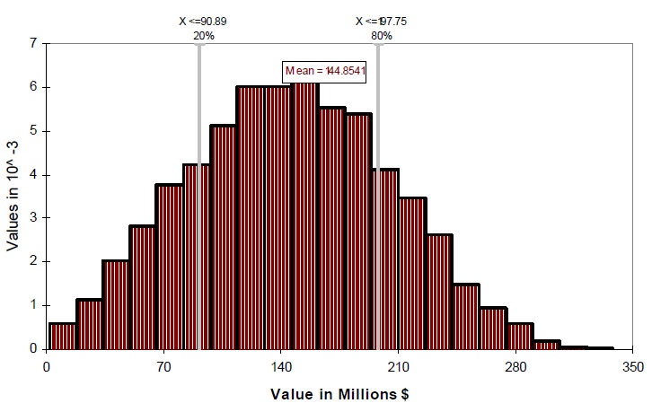
Exhibit 30 Distribution of Net Benefits (Present Value) Credit River– 16 Mile Creek – Streams
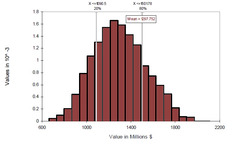
4.1.2 Toronto Area
Exhibit 31 presents the present value of net benefits of habitat protection and restoration for Toronto Area. As shown, the present value of net benefits for wetlands range from $70.58 to $117.02 million with a most likely estimate of $93.96. For the stream system habitat, the present value of net benefits for wetlands range from $397.68 to $1,813.23 million with a most likely estimate of $1,108.69.
Exhibit 32 and Exhibit 33 present the probability distribution of net benefits of wetlands and stream system restoration and protection for Toronto Area. In the case of wetlands, Exhibit 32 shows that all of the likely outcomes of the net benefit are positive. Therefore, although there is a risk that the net benefit of wetland protection and restoration will be negative, it is likely a small risk. In the case of stream systems, Exhibit 33 shows that there is an 8.6% probability that the present value of net benefits will be negative according to this analysis. This result is not surprising because of the high costs of land acquisition and the wide range in annual benefits that was estimated in Section 3.1.3 using the two valuation methods.
In further sensitivity analysis, the variables that have the greatest impact on the present value on net benefits of wetlands are the annual value of other wetlands (positive) and the social discount rate (negative). In the case of stream systems, the variables that have the greatest impact on net benefits are the total value of benefits each year (positive) and the costs of purchasing land (negative).
| Low * | Mean * | High * | ||
|---|---|---|---|---|
| Wetlands | Benefits | $73,270,000 | $96,790,000 | $119,730,000 |
| Wetlands | Costs | $2,430,000 | $2,830,000 | $3,240,000 |
| Wetlands | Net Benefits | $70,580,000 | $93,960,000 | $117,020,000 |
| Wetlands | Benefit Cost Ratio | 25.3 | 35.2 | 44.3 |
| Stream Systems | Benefits | $1,958,200,000 | $2,598,710,000 | $3,217,500,000 |
| Stream Systems | Costs | $1,156,510,000 | $1,490,020,000 | $1,826,020,000 |
| Stream Systems | Net Benefits | $397,680,000 | $1,108,690,000 | $1,813,230,000 |
| Stream Systems | Benefit Cost Ratio | 1.3 | 1.9 | 2.5 |
| Total | Benefits | $2,056,860,000 | $2,695,500,000 | $3,317,530,000 |
| Total | Costs | $1,159,120,000 | $1,492,850,000 | $1,828,680,000 |
| Total | Net Benefits | $488,900,000 | $1,202,650,000 | $1,910,020,000 |
* These result show combinations of outcomes and the columns are not additive. That is, the low column may be a combination of a low cost and a high benefit for different category and any number of combinations in between.
Exhibit 32 Distribution of Net Benefits (Present Value) for Toronto Area – Wetlands
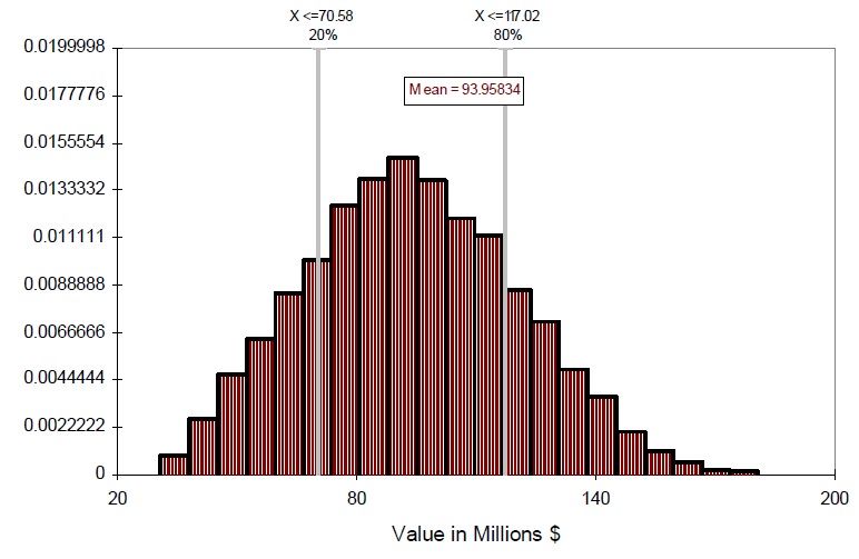
Exhibit 33 Distribution of Net Benefits (Present Value) for Toronto Area – Streams
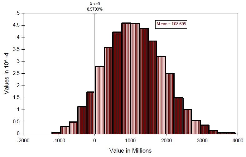
4.1.3 Prince Edward Bay
Exhibit 34 presents the present value of net benefits of habitat protection and restoration for Prince Edward Bay. As shown, the present value of net benefits for wetlands range from $285.41 to $322.15 million with a most likely estimate of $358.29. For the stream system habitat, the present value of net benefits for wetlands range from $886.47 to $1,090.34 million with a most likely estimate of $988.08.
Exhibit 35 and Exhibit 36 present the probability distribution of net benefits of wetlands and stream system restoration and protection for Prince Edward Bay. As can be seen, all of the likely outcomes of the net benefit are positive. Therefore, although there is a risk that the net benefit of habitat protection and restoration will be negative, it is likely a small risk.
In further sensitivity analysis, the variables that have the greatest impact on the present value on net benefits of wetlands are the social discount rate (negative) and the annual value of other wetlands (positive). In the case of stream systems, the variables that have the greatest impact on net benefits are the discount rate (negative) and the total value of benefits each year (positive).
| Low * | Mean * | High * | ||
|---|---|---|---|---|
| Wetlands | Benefits | $312,470,000 | $349,340,000 | $385,580,000 |
| Wetlands | Costs | $23,480,000 | $27,190,000 | $30,850,000 |
| Wetlands | Net Benefits | $285,410,000 | $322,150,000 | $358,290,000 |
| Wetlands | Benefit Cost Ratio | 10.9 | 13.0 | 14.9 |
| Stream Systems | Benefits | $689,300,000 | $763,430,000 | $837,380,000 |
| Stream Systems | Costs | $84,760,000 | $97,490,000 | $110,250,000 |
| Stream Systems | Net Benefits | $592,540,000 | $665,930,000 | $739,540,000 |
| Stream Systems | Benefit Cost Ratio | 6.7 | 8.0 | 9.2 |
| Total | Benefits | $1,009,230,000 | $1,112,760,000 | $1,214,910,000 |
| Total | Costs | $111,230,000 | $124,680,000 | $137,820,000 |
| Total | Net Benefits | $886,470,000 | $988,080,000 | $1,090,340,000 |
* These result show combinations of outcomes and the columns are not additive. That is, the low column may be a combination of a low cost and a high benefit for different category and any number of combinations in between.
Exhibit 35 Distribution of Net Benefits (Present Value) for Prince Edward Bay - Wetlands
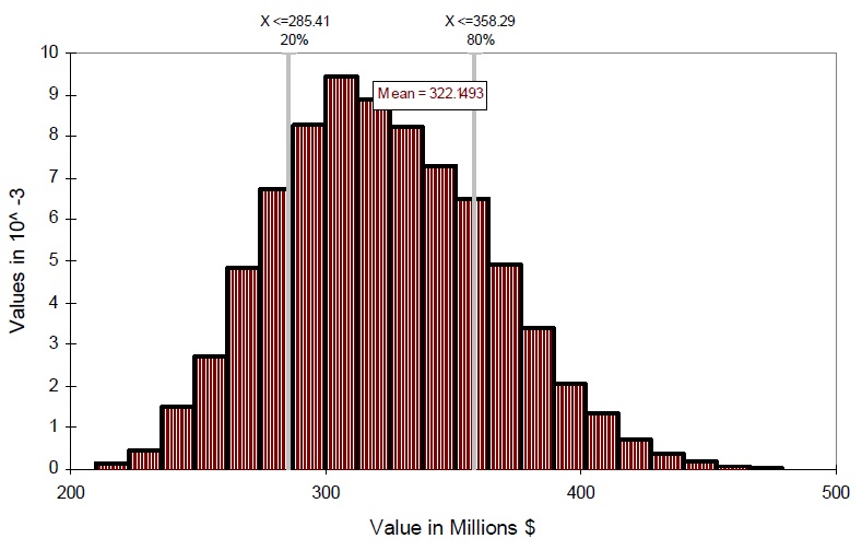
Exhibit 36 Distribution of Net Benefits (Present Value) for Prince Edward Bay – Streams
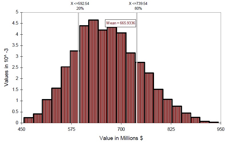
4.1.4 Per hectare Benefits and Costs
This section reports the results of the previous section on a per hectare basis. This is done so that a more useful comparison of the costs and benefits of habitat protection and restoration across the three watersheds can be made.
Exhibit 37 summarizes the present value of benefits and costs of restoring and protecting of wetlands for the three watersheds on a per hectare basis. As shown, both the present value of benefits and costs per hectare of wetland are highest in the Toronto Area watershed. This result is not surprising. On the benefits side, Toronto Area has the highest population density, the lowest abundance of neighbouring wetlands and the highest degree of human pressure. All these factors increase the per hectare value of wetlands. On the costs side, land prices are highest in the Toronto Area and therefore, purchasing land for habitat protection is expensive.
On the other hand, both the present value of benefits and costs per hectare of wetland are lowest in Prince Edward Bay. Prince Edward Bay has a low population density, a lot of neighbouring wetlands and medium levels of human pressure. All these factors decrease the per hectare value of wetlands. In addition, land prices are the lowest in Prince Edward Bay and therefore, purchasing land for habitat protection is relatively cheap compared to the other two watersheds.
The present value of benefits and costs of wetlands in Credit River – 16 Mile Creek is between these two cases.
We can conclude that in all three watersheds, the present value of benefits per hectare of wetland is much higher than the present value of costs per hectare, as shown in Exhibit 37. The average benefit-cost ratio across all three watersheds is 24.
| Watershed | Benefits - Low | Benefits - Mean | Benefits - High | Costs - Low | Costs - Mean | Costs - High |
|---|---|---|---|---|---|---|
| Credit River – 16 Mile Creek | $1,031,376 | $1,630,129 | $2,213,999 | $62,871 | $70,694 | $78,582 |
| Toronto Area | $2,983,199 | $3,940,660 | $4,874,582 | $98,776 | $115,384 | $131,850 |
| Prince Edward Bay | $321,262 | $359,168 | $396,431 | $24,141 | $27,952 | $31,721 |
Exhibit 38 summarizes the present value of benefits and costs of restoring and protecting of stream systems for the three watersheds on a per hectare basis. Similar to the wetland values shown directly above, both the present value of benefits and costs are highest in Toronto Area, and lowest in Prince Edward Bay.
| Watershed | Benefits - Low | Benefits - Mean | Benefits - High | Costs - Low | Costs - Mean | Costs - High |
|---|---|---|---|---|---|---|
| Credit River – 16 Mile Creek | $69,446 | $75,958 | $82,442 | $27,255 | $31,210 | $35,131 |
| Toronto Area | $87,105 | $115,597 | $143,122 | $51,444 | $66,279 | $81,226 |
| Prince Edward Bay | $56,631 | $62,720 | $68,796 | $6,964 | $8,010 | $9,058 |
We can conclude that based on our analysis, wetlands have much higher present value if economic benefits per hectare compared to stream systems. This is true in all three of the watersheds considered in this analysis. This is a common finding in the ecosystem service valuation literature (Troy and Bagstad; Kennedy and Wilson 2009).
4.1.5 Non-monetized Benefits
Intangible benefits are those that cannot be assigned a monetary value. These include benefits that are not quantified, and benefits that are quantified, but not monetized. This may be the case when data is not available or if it is not clear how to quantify/measure the value even with data.
In the case of wetlands, Exhibit 49 in Appendix D provides an overview of the goods and services that are included and not included in the meta-analyses. Important wetland services that are not included in this analysis are non-use values, sediment retention and local climate regulation. The benefits accounted for stream systems are derived from several studies relying on contingency valuation. The valuation categories are sometimes generalized, so there is some uncertainty as to which specific benefits are/are not included. For instance, recreation could be sub-divided into several benefit categories including fishing, boating, hiking, biking, picnicking, etc..
The value categories that are definitely not accounted for are non-use values and option values. Non-use values include existence and bequest values. For the former, the benefit value is derived from the knowledge that habitat is protected/restored, even if those who attribute this value do not directly live in or visit the area. Many people who will never visit the Ontario Great Lakes region place value on its protection, or on the protection of its populations of endangered, threatened, or highly valued species of birds, fish, and other animals. In other words, people have demonstrated willingness-to-pay to protect or improve areas that are of no direct use to them, simply for the benefit derived from knowing these areas exist in their natural ecological state. The benefit of bequest values comes from the knowledge that habitat will be protected for the potential use of future generations. Option value is captured by the possibility of deriving benefits from other use-values generated by habitat protection. Therefore, the value comes from the attractive option of using protected or restored habitats in the future (Tietenberg, 2006; Austin et al., 2007).
Non-use values have been estimated to account for to 60% to 80% of total economic value (Freeman, 1979). In fact, in recognition of the probability of high values for non-use benefits, until recently, the EPA added a non-use benefit of equal to one-half of the total recreational use benefits (EPA, 2000).
Non-use values, in addition to the other non-monetized impacts in our analysis, could add significantly to the total welfare benefit value of habitat protection and restoration.
4.2 Coastal Shoreline Discussion
In a comprehensive review and assessment of nonmarket valuation studies that are relevant for Southern Ontario, Troy and Bagstad (2009) categorized valuation estimates according to land cover types. The only separate shoreline land cover types included in the analysis was wetlands and beaches. Therefore, the bottom line is that the existing economics literature cannot provide accurate and unique estimates of the shoreline habitat type as defined in the Conservation Blueprint. The fact that the literature does not reflect values for this type of habitat likely reflects the on-the-ground reality that coastal shoreline habitat protection faces significant challenges due to a poor ability to compete with other coastal shoreline uses, in particular beach use. The plight of the endangered Piping Plover illustrates this situation; despite its endangered status, this species is protected on a nest-by-nest basis with little impact on beach use by humans. Valuation of this habitat type is difficult in the absence of clear demonstration by Canadians that its protection is worthwhile.
5.0 Summary and Implications
5.1 Summary of Results
Our results indicate that the benefit cost ratio for wetland protection and restoration ranges from 13.0 for Prince Edward Bay to 35.2 for Toronto Area. For stream system restoration, the cost benefit ratio ranges from 1.9 for Toronto Area to 8.0 for Prince Edward Bay.
Both the present value of benefits and costs per hectare of wetland are highest in the Toronto Area watershed. This result is not surprising. On the benefits side, Toronto Area has the highest population density, the lowest abundance of neighbouring wetlands and the highest degree of human pressure. All these factors increase the per hectare value of wetlands. On the costs side, land prices are highest in the Toronto Area and therefore, purchasing land for habitat protection is expensive.
On the other hand, both the present value of benefits and costs per hectare of wetland are lowest in Prince Edward Bay. Prince Edward Bay has a low population density, a lot of neighbouring wetlands and medium levels of human pressure. All these factors decrease the per hectare value of wetlands. In addition, land prices are the lowest in Prince Edward Bay and therefore, purchasing land for habitat protection is relatively cheap compared to the other two watersheds. The present value of benefits and costs of wetlands in Credit River – 16 Mile Creek is between these two cases.
For all three wetlands, we can conclude that the present value of benefits per hectare of wetland is much higher than the present value of costs per hectare. Important wetland services that are not included in this analysis are non-use values, sediment retention and local climate regulation. Value categories that are not accounted for in the stream habitat valuation are non- use values and option values. Non-use values include existence and bequest values. Non-use values have been estimated to account for to 60% to 80% of total economic value (Freeman 1979) and, in addition to the other non-monetized impacts in our analysis, could add significantly to the total welfare benefit value of habitat protection and restoration.
Caution is needed in interpreting our results for a number of reasons. One of the most important is that, in the case of stream systems, we apply constant marginal values for habitat types across large areas of habitat. In effect, we assume that habitats exhibit constant returns to scale in habitat size with respect to benefits. To the extent that the benefits derived from habitat exhibit decreasing returns to scale in habitat size, our estimates will overestimate the benefits of habitat protection and restoration. As discussed in this report, wetland habitats experience these types of decreasing returns to scale in habitat size (Brander et al., 2009; Ghermandi et al., 2010). On the other hand, to the extent that the benefits derived from habitat exhibit increasing returns to scale in habitat size, our estimates will underestimate the benefits of habitat protection and restoration. A recent contingent valuation study of stream restoration by Holmes et al. (2004) provides some empirical evidence for increasing returns to scale in habitat size. Respondents were found to be willing to pay a premium for total restoration of the ecosystem relative to a partial restoration (Holmes et al., 2004). Changing this simplifying assumption on the constancy of marginal values across habitat sizes will change the quantitative results derived in this analysis.
This study focuses specifically on three tertiary Lake Ontario watersheds; therefore the results presented in the report are specific to these watersheds. However, this approach to cost- benefit analysis can be applied to any watershed, given that the appropriate input data are available. In addition, the results of this analysis provide some indication of the expected magnitudes of costs and benefits in other watersheds.
In the case of wetlands, we can generalize and state that watersheds with high population densities, intense human pressure and low wetland abundance will have higher values of benefits compared to watersheds with low population densities, medium human pressure and high neighbouring wetland abundance. Of course, although the economic benefits are lower in more rural watersheds, so are the costs of purchasing the land for habitat protection.
5.2 Policy Implications
The most significant policy implication emerging from this analysis is that there are positive economic returns on restoration and protection of all habitat types evaluated. Thus, policy instruments designed to undertake and encourage habitat protection and restoration are warranted, particularly in more densely populated regions. This is true even though costs of land securement are also higher in and around urban areas.
It was not possible to evaluate coastal habitats that were not wetlands. There are no apparent market drivers and little public awareness to ensure these types of habitat and the species within them continue to have a viable existence. Therefore government interventions for these types of habitat (e.g. sandy coastal flats) are imperative for their successful protection or restoration.
5.3 Implications for Future Analysis
As previously discussed, this study was narrowly scoped due to time and budget constraints. Two important scoping issues, which have implications for future analysis, are that the study looked only at Lake Ontario watersheds and that the study was based on the conservation goals of the Conservation Blueprint. Throughout this study process, it has been noted that the data in the Conservation Blueprint is dated and possibly inaccurate with respect to conservation lands. However, the cost-benefit approach employed here and the valuation methods could be applied to other watersheds, with other intervention portfolios, using other (similar) data with respect to additional area needed for conservation. In other words, studies with updated conservation targets, and needed information on the additional area required to meet the habitat/biodiversity targets with the related portfolio of intervention strategies, could readily be referenced for application of this cost-benefit analysis approach to determine the total costs and total benefits for a watershed.
This study focused specifically on three tertiary Lake Ontario watersheds; therefore the results presented in the report are specific to these watersheds. However, this approach to cost- benefit analysis can be applied to any watershed, given that the appropriate input data is available. In addition, the results of this analysis provide some indication of the expected magnitudes of costs and benefits in other watersheds. In the case of wetlands, we can generalize and state that watersheds with high population densities, intense human pressure and low wetland abundance will have higher values of benefits compared to watersheds with low population densities, medium human pressure and high neighbouring wetland abundance. Of course, although the economic benefits are lower in more rural watersheds, so are the costs of purchasing the land for habitat protection. This study includes two interventions: land securement and restoration. Additional work is needed to develop the methodologies for valuation of other interventions, such as use of land easements for habitat protection.
Other key issues arising from this report for potential future analysis include:
- There is a significant need for recent, Canadian-specific primary valuation studies. This information is particularly important given the recent empirical research that suggests that Canadians may have a substantially different WTP for SWQ improvements compared to Americans.
- To conduct a more general Great Lakes Basin cost benefit analysis à la America’s North Coast report, there needs to be a fully-costed Canadian Great Lakes Action Plan to be evaluated.
- In sum, the current analysis provides an important methodological approach to estimating the economic value of habitat improvements. As additional information improves the underlying scientific knowledge of the importance of habitats of all kinds for the health of the Great Lakes ecosystem, these additional considerations can be formally included in future analyses.
1 Wichert, G.A., K.E. Brodribb, B.L. Henson, and C. Phair, Great Lakes Conservation Blueprint for Aquatic Biodiversity, Volume 1, Nature Conservancy Canada, Natural Heritage Information Centre, Ontario Ministry of Natural Resources, 2005.
2 Exhibit 5 in Section 2.2.4 provides the full list of wetland services considered in these two meta-analyses.
3 Exhibit 6 and the text in Section 2.2.4 provides the full list of wetland services considered in these two studies
4 Roni (2005) lists a number of such studies.
5 In this study, “upland” refers to the non-riparian area adjacent to the stream systems (i.e., from 30 m to 300 m).
6 To avoid confusion regarding the actual geographic area of this tertiary watershed, the Humber-Don Rivers watershed (2HC) is referred to as the “Toronto Area” watersheds in this study.
7 There exist multiple theories of value and therefore, there are many different approaches to valuation. The two main valuation paradigms are the economic method selected in this report and biophysical methods (Pascual and Muradian, 2010). Biophysical methods measure the physical cost of producing goods and services and use a “cost of production” perspective for valuation (Pascual and Muradian, 2010).
8 It is important to note that not all ecosystem services are indirect uses and not all indirect uses are ecosystem services. Clearly, all the goods and services in the Great Lakes ultimately come from the ecosystem. In deciding the organization and wording of this section, we choose to name the indirect use value section as ecosystem services to communicate the more natural foundations of these services.
9 All values presented in this report have been converted to 2009 Canadian dollars, unless stated otherwise. This conversion was done using Statistics Canada data on the Canadian Price Index (v41693271). Data accessed from CANSIM using CHASS. Values were converted into Canadian dollars using Purchasing Power Parity (PPP) conversion factors from the OECD.
10 US EPA, Guidelines for Preparing Economic Analysis, EPA 240-R-00-003, 2002.
11 Peli et al., Economic Analysis of Investment Operations. World Bank Institute, 2002.
12 The Green Book, Appraisal and Evaluation in Central Government, UK.
13 It has been noted that the areas identified as Conservation Authority lands may be underrepresented in the Blueprint data. Please see Limitations in Section 3.4.
14 This assumption likely overestimates the value of converting areas currently not under natural cover to protected habitat because some areas not in natural cover are nevertheless producing some, though much lower, ecosystem values even in an unprotected state.
15 Some academics include a new third approach: preference calibration. Preference calibration uses information from the study site to identify parameters that identify underlying preferences. These preference relationships are then used to estimate benefits at the policy site. This relatively new transfer method has limited use in environmental economics because it requires the time-consuming specification of the structure of preferences.
16 The number of studies by valuation method for each wetland service included in Brander et al. (2010) is provided in Appendix D, Exhibit 49.
17 We use population and wetland abundance data at the watershed level as proxies for the relevant variables in the regression equation. Because both of these variables enter the regression equation as a function of their natural logs, this assumption is not expected to impact our results to a large degree. We assess the benefits for this 50 km radius to maintain consistency with the underlying meta-analyses.
18 It should be noted that these are average sizes of the whole wetland, not only the part that needs to be protected and possibly restored.
19 Although the US WTP estimates from Loomis et al. (2000) are adjusted downward for the Canadian context, the meta-analysis values of Brander et al. (2010) and Ghermandi et al. (2009) are not adjusted. The main reason is that these wetland service studies include value estimates from many different countries and there is no clear empirical basis for adjusting these wetland values across countries. For example, we do not know if Canadians would have a higher WTP for wetlands than reported in the two meta-analyses or a lower WTP. As noted by Johnston and Thomassin (2010), cross country comparisons of WTP estimates for environmental goods and services is rarely done and the limited evidence provides little guidance.
21 The RiskTrigen function was chosen over alternative distribution functions (normal, gamma etc.) for its simplicity, and because it does not have ‘tails’. That is to say, the RiskTrigen function does not allow variable values that are far outside the low and high estimated values.
22 The one exception to this is the population density variable. For this variable we use the average number of people per square kilometre as calculated in Section 3.1.3.
23 In the case of Prince Edward Bay, because the two methods derive very similar cost estimates ($6,843 using the first method and $6,472 using the second method), we vary the average costs of the two methods by 25% to arrive at a high and low estimate.
24 The Canadian cost data included project costs but none of the Canadian projects had additional O&M costs.
25 This calculation is done using the central discount rate of 3.5%.
26 The data is limited in two senses. The first limitation is that the Conservation Blueprint does not provide information on the underlying wetland quality as it relates to restoration needs. The second limitation is that the restoration cost estimates used in this analysis are not linked to wetland quality before the project was undertaken. Taken together, these limitations imply that we are able to assess the quantitative restoration needs (how much additional area of wetlands need to be actively restored?) of the three watersheds based on the approach outlined in Section 3.1.1, but not the restoration needs based on quality of wetlands.
27 Statistics Canada 2006 Community Profiles,
28 We need to first convert the income per capita to 2003 US dollars for consistency with the meta-analyses. Of course, we then convert the values derived from the meta-analyses that are in 2003 US dollars to 2009 Canadian dollars.
29 In addition, these two wetland sizes allow us to examine the effect of wetland size on wetland value using the meta-analyses.
30 These variables account for alterations in the natural hydrologic regime of the wetland, whether the wetland is located in an urban or rural setting and the wetland’s protection status.
31 However, it is important to remember that a common critique of environmental meta-analyses is that not all of the underlying primary studies define the wetland services in the same way. In the jargon of the environmental meta-analysis literature, this limitation is referred to as a lack of commodity consistency. This limitation makes it difficult to robustly evaluate the relative contribution of each wetland service to the total WTP in frontier empirical work such as the meta-analyses of Brander and Ghermandi.
32 This average is calculated as the simple average of the wetland values from references identified in Appendix C.
33In general, most projects aim to restore more than one habitat type. For example, the 98 projects that restore wetlands also restore or improve 4,670 acres of open water/nearshore habitat, 44,477 acres of riverine/riparian habitat, and 107,429 acres of coastal/upland habitat. This is why the total reported costs of all projects is not the simple sum of the total cost per habitat type. In addition, these habitat restoration projects work to achieve the broader goals of the Great Lakes Regional Collaboration Strategy such as non-point source pollution control and invasive species reduction.
Appendix A Vyn’s Land Pricing Model
| Coefficients | Mean values | |
|---|---|---|
| Constant | -15.6608 |
| Coefficients | Mean values | |
|---|---|---|
| Lot Size (ln) (acres) | -0.4346*** | 63.4833 |
| Class 1 land | 0.67*** | 0.2871 |
| Class 2 land | 0.4031*** | 0.3233 |
| Wooded area | -0.2476*** | 0.0983 |
| Organic Soil | -0.2565 | 0.0027 |
| Heat units (ln) | 3.1834*** | 2736.812 |
| Orchard/Vineyard | 0.8136*** | 0.0114 |
| Coefficients | Mean values | |
|---|---|---|
| Population Density (ln) | 0.2845*** | 143.8736 |
| Growth rate | 0.0542*** | 1.3132 |
| Water/sewer | 0.0489* | 0.339 |
| Coefficients | Mean values | |
|---|---|---|
| Distance to GTA km (ln) | -0.2143*** | 61.8195 |
| Distance to town km (ln) | -0.083*** | 17.5493 |
| Northumberland | -0.3692*** | |
| Durham | -0.1699* | |
| York | 0.4909*** | |
| Peel | 0.357*** | |
| Halton | 0.1182 | |
| Hamilton | -0.8987*** | |
| Brant | -0.5076*** | |
| Bruce | 0.016 | |
| Dufferin | 0.1829** | |
| Grey | -0.0601 | |
| Haldimand-Norfolk | -0.8171*** | |
| Huron | 0.1903** | |
| Kawartha | -0.3777*** | |
| Niagara | -0.9714*** | |
| Oxford | 0.1744** | |
| Perth | 0.4632*** | |
| Peterbourough | -0.1628* | |
| Simcoe | 0.1397** | |
| Waterloo | 0.3689*** |
Notes: Wellington County is the omitted location variable.
* Indicates that the coefficient is significantly different from zero at the 10%
** Indicates that the coefficient is significantly different from zero at the 5%
*** Indicates that the coefficient is significantly different from zero at the 1%
Appendix B Costs of Habitat Interventions
| Project | Wetland Area (acres) | Project Cost | Annualized project cost | Annual cost per hectare |
|---|---|---|---|---|
| Coastal Wetlands Rehabilitation | 10 | $5,536,597 | $320,183 | $82,134 |
| Re-Introduction of Southern Wild Rice Into Cootes Paradise | 1 | $257,097 | $14,870 | $59,504 |
| Franklin Garden Demonstration Wetland | 1 | $321,644 | $18,599 | $37,211 |
| Youth and Community Greening the Rouge River Watershed | 21 | $1,627,600 | $94,123 | $11,738 |
| Humber Bay Shores Butterfly Meadow | 2 | $109,034 | $6,306 | $8,413 |
| Rouge Watershed Wetland Creation Initiative: Phase 3 | 17 | $931,227 | $53,851 | $7,695 |
| Lower Don River - Habitat Restoration Projects | 24 | $825,195 | $47,719 | $4,822 |
| Milne Park Natural and Cultural Heritage Restoration | 3 | $96,207 | $5,561 | $3,976 |
| Granger Greenway Habitat Enhancement | 8 | $225,984 | $13,065 | $3,868 |
| Spencer Creek Fisheries Projects | 9 | $201,966 | $11,681 | $3,338 |
| Toronto Island Sand Dune Restoration | 2 | $52,402 | $3,031 | $3,032 |
| Humberwood Bird Habitat Enhancement Project | 1 | $8,051 | $467 | $1,167 |
| Hamilton Harbour Watershed Stewardship Project | 29 | $180,405 | $10,434 | $897 |
| Grindstone Creek & Cootes Paradise Rehabilitation Project | 667 | $3,392,210 | $196,176 | $728 |
| Bruce’s Mill Dam Decommissioning & Wildlife Habitat Enhancement Project | 7 | $28,521 | $1,647 | $550 |
| Claireville Natural Area Enhancement 46 | 46 | $60,317 | $3,487 | $185 |
(Source: International Lake Ontario-St. Lawrence River Study Board (2006))
Note: The total project costs are annualized using a 4% discount rate and a 30 year repayment period. These costs do not include the cost of labour that was provided by volunteers.
| Open and Near-shore Waters | Wetlands | Riparian | Costal and Upland | |
|---|---|---|---|---|
| Number of Projects | 41 | 98 | 114 | 98 |
| Acres Potentially Restored | 4,858 | 62,282 | 52,222 | 186,989 |
| Total Cost per Habitat Type ($2009) | $239,833,000 | $485,885,000 | $423,329,000 | $181,238,000 |
| Total Reported Costs of all Projects ($2009) | $916,765,000 | |||
(Source: USACE, 2008)
| Size of Land Purchases | Total Purchase costs($2009) | Costs per hectare ($2009) |
|---|---|---|
| 17,064 hectares | $21,939,150 | $1,285.7 |
(Source: Sverrisson (2008))
Additional information
The cost data presented below, although very useful for this type of study, was provided too late to be included in our analysis. This type of data is important to obtain during the early stages of the analysis, as it is used as input to determine the final costs per hectare. That said, this data was still informative for cross-checking and validation.
| Restoration Measure | Cost per Unit | Unit | Lifetime |
|---|---|---|---|
| Instream barrier removal | $58,487 | barrier | 50 |
| Channel restoration - major | $1,170 | m | 50 |
| Channel restoration - minor | $585 | m | 50 |
| bank vegetation | $117 | m | 50 |
| Project Type | Total Cost (millions) | Total Length (km) | Cost/km | Cost/m |
|---|---|---|---|---|
| Aesthetics/recreation/education | $4.8 | 12.87 | $372,960 | $501 |
| Bank stabilization | $19.4 | 151.28 | $128,239 | $172 |
| Channel reconfiguration | $6.2 | 43.45 | $142,693 | $192 |
| Dam removal/retrofit | $9.0 | 0.03 | $300,000,000 | $403,342 |
| Fish passage | $8.3 | 4.18 | $1,985,646 | $2,670 |
| Floodplain reconnection | $6.3 | 8.69 | $724,971 | $975 |
| Flow modification | $1.3 | 3.86 | $336,788 | $453 |
| In-stream habitat improvement | $32.2 | 65.98 | $488,027 | $656 |
| In-stream species management | $7.5 | 0.8 | $9,375,000 | $12,604 |
| Land acquisition | $21.5 | 0.4 | $53,750,000 | $72,265 |
| Riparian management | $18.0 | 2146.86 | $8,384 | $11 |
| Storm water management | $10.7 | 16.09 | $665,009 | $894 |
| Water quality | $84.0 | 1170 | $71,795 | $97 |
| Project Name | Description | Cost/m |
|---|---|---|
| Don River restoration - 1 | mitigation using planted fieldstone and bank reshaping along 120 m reach, both sides | $3000/m |
| Don River restoration - 2 | As above – 230 m reach, one side | $1850/m |
| Credit River relocation and restoration | 1.1km reach, planted fieldstone, j hooks and grade control structure, restoration both sides | $1275/m |
| 16 Mile Creek realignment and Redside Dace Habitat restoration | 600 m reach, 60 m wide valley corridor, 1 m wide trib. Both sides using sod blocks and harvested stock | $1250/m |
| Toogood Pond Fishway | Purpose built fishway to by-pass a dam 65 m | $5385/m |
| Rouge River erosion site 5 | Planted fieldstone and grade control structure 25 m (higher cost because of remote site in urban area) | $5000/m |
| Highland Creek stabilization | 225 m reach, grade control structure, reinforced earth embankment, realignment, bioengineering and fieldstone shoulder treatments | $4890/m |
| Pine Creek stabilization and Dam removal | 160 m reach, removal of low head dam, full channel reconstruction and bioengineering, both sides | $2500/m |
Appendix C Benefits of Habitat Interventions
| Source | Location | Wetland Type | Annual Wetland Value per Hectare |
|---|---|---|---|
| Tejani and Muir (2003) | Hamilton-Halton Watershed | Wetland | $26,561 |
| Bruenig (2003) | Massachusetts | Wetland | $54,059 |
| Olewiler (2004) | Grand River Watershed, | Wetland, low estimate | $13,172 |
| Olewiler (2004) | Fraser valley, BC | Wetland, high estimate | $55,324 |
| David Suzuki Foundation (2008) | Ontario Greenbelt | Wetland | $15,132 |
| Wilson (2008) | Lake Simcoe Watershed | Shallow water | $15,280 |
| Wilson (2008) | Lake Simcoe Watershed | Bog | $15,649 |
| Wilson (2008) | Lake Simcoe Watershed | Marsh | $15,377 |
| Wilson (2008) | Lake Simcoe Watershed | Swamp | $15,175 |
| Wilson (2008) | Lake Simcoe Watershed | Fen | $16,006 |
| Troy and Bagstad (2009) | Southern Ontario | Nonurban/non-coastal | $15,211 |
| Troy and Bagstad (2009) | Southern Ontario | Urban/Suburban | $161,844 |
| Troy and Bagstad (2009) | Southern Ontario | Great Lakes coastal | $14,800 |
| Kennedy and Wilson (2009) | Credit Valley Watershed | Wetland | $32,507 |
| Source | Location | Habitat Type | Benefits Included in the Analysis | Habitat Value per Hectare ($2009) |
|---|---|---|---|---|
| Troy and Bagstad (2009) | Southern Ontario | Forest adjacent to a stream | Recreation | $560 |
| Troy and Bagstad (2009) | Southern Ontario | Forest adjacent to a stream | Habitat refugium and Biodiversity | $133 |
| Troy and Bagstad (2009) | Southern Ontario | Forest adjacent to a stream | Atmospheric Regulation | $995 |
| Troy and Bagstad (2009) | Southern Ontario | Forest adjacent to a stream | Soil Retention/Erosion Control | $781 |
| Troy and Bagstad (2009) | Southern Ontario | Forest adjacent to a stream | Water Quality/nutrient & waste regulation | $614 |
| Troy and Bagstad (2009) | Southern Ontario | Forest adjacent to a stream | Water Supply/Regulation | $1,323 |
| Troy and Bagstad (2009) | Southern Ontario | Forest adjacent to a stream | Disturbance Avoidance | $148 |
| Troy and Bagstad (2009) | Southern Ontario | Forest adjacent to a stream | Total | $4,564 |
| Troy and Bagstad (2009) | Southern Ontario | River (open water) | Recreation | $8,678 |
| Troy and Bagstad (2009) | Southern Ontario | River (open water) | Other Cultural | $25 |
| Troy and Bagstad (2009) | Southern Ontario | River (open water) | Habitat refugium and Biodiversity | $10 |
| Troy and Bagstad (2009) | Southern Ontario | River (open water) | Water Quality/nutrient & waste regulation | $33,996 |
| Troy and Bagstad (2009) | Southern Ontario | River (open water) | Water Supply/Regulation | $12,991 |
| Troy and Bagstad (2009) | Southern Ontario | River (open water) | Total | $55,699 |
| Troy and Bagstad (2009) | Southern Ontario | Urban/suburban river (open water) | Recreation | $173,148 |
| Troy and Bagstad (2009) | Southern Ontario | Urban/suburban river (open water) | Aesthetic and Amenity | $243 |
| Troy and Bagstad (2009) | Southern Ontario | Urban/suburban river (open water) | Water Quality/nutrient & waste regulation | $45,889 |
| Troy and Bagstad (2009) | Southern Ontario | Urban/suburban river (open water) | Water Supply/Regulation | $17,737 |
| Troy and Bagstad (2009) | Southern Ontario | Urban/suburban river (open water) | Total | $237,013 |
| Kennedy and Wilson (2009) | Credit Valley Watershed | Riparian Forests | Atmospheric Regulation | $19,316 |
| Kennedy and Wilson (2009) | Credit Valley Watershed | Riparian Forests | Waste Treatment | |
| Kennedy and Wilson (2009) | Credit Valley Watershed | Riparian Forests | Water Purification | |
| Kennedy and Wilson (2009) | Credit Valley Watershed | Riparian Forests | Soil Retention | |
| Kennedy and Wilson (2009) | Credit Valley Watershed | Riparian Forests | Habitat | |
| Kennedy and Wilson (2009) | Credit Valley Watershed | Riparian Forests | Recreation |
| Loomis et al. (2000) | Holmes et al. (2004) | |
|---|---|---|
| Study Location | Platte River, Colorado | Little Tennessee River, North Carolina |
| Ecosystem services | Dilution of wastewater | Ecosystem integrity (index of ecosystem naturalness) |
| Ecosystem services | Natural purification of water | Water purification (water clarity) |
| Ecosystem services | Erosion control | Erosion control |
| Ecosystem services | Habitat for fish and wildlife | Habitat for fish (abundance of game fish), habitat for wildlife (wildlife habitat in buffer zones) |
| Ecosystem services | Recreation | Recreational uses (allowable water uses) |
| Area of restoration | 121,406 ha of conservation easements along 72 km of river | 9.6 km of river restoration |
| Annual WTP per household | $375 ($5.21 per km of river restored) | $79 ($8.23 per km of river restored) |
Appendix D Wetland Valuation Meta-Analyses Results
There have been four published meta-analyses of wetland valuation studies:
- Brouwer et al. (1999) conducted a meta-analysis of 92 value observations from 30 studies of temperate climate zone wetlands that employed the contingent valuation literature.
- Woodward and Wui (2001) analyzed 65 value observations from 39 North American and European wetland valuation studies. This analysis included studies that employed a variety of valuation techniques other than contingent valuation (hedonic pricing, travel cost method, etc.).
- Brander et al. (2006) included 215 value observations from 80 studies that included both tropical and temperate wetland types. This meta-analysis also included socio- economic and demographic variables in the regression equation.
- Ghermandi et al. (2007) analyzed 383 value observations from 166 studies. In addition to socio-economic and demographic variables, man-made wetlands are included for the first time.
Clearly meta-analyses of wetland valuation studies have expanded in scope and scale over the last ten years. In addition, two recent (unpublished) meta-analyses have built on the previous results and these are most useful for our analysis. Ghermandi et al. (2009) expands the number of value observations in Ghermandi et al. (2007) to include 418 observations from 189 studies. In addition, Brander et al. (2010) analyzed 264 value observations from temperate climate zone wetlands. Results of these two studies are presented below.
Exhibit 49 Number of Studies by Valuation Method for each Wetland Service (Brander et al. (2010)
| Category | Wetland Service | Valuation Methods |
|---|---|---|
| Cultural | Ameaity and aesthetics | CVM (22), HP (5), TCM (5) |
| Cultural | Non-consumptive recreational activities | CVM (44),TCM (18) |
| Cultural | Appreciation of uniqueness to cultural/heritage | N/A |
| Cultural | Educational | N/A |
| Cultural | Recreational hunting | CVM (14),TCM (21) |
| Cultural | Recreational fishing | CVM (22),TCM (15) |
| Cultural | Non-use values | N/A |
| Supporting | Biodiversity | CVM (23), choice experiment (6), market prices(5) |
| Supporting | Support of pollinators | N/A |
| Provisioning | Commercial fishing and hunting | Market prices (18), NFI (18), CVM (10) |
| Provisioning | Harvesting of natural materials | Market prices (18), NFI (11), CVM (8) |
| Provisioning | Fuel Wood | Market prices (7), NFI (4) |
| Provisioning | Surface and ground water | Replacement cost (15) |
| Regulating | Flood control and storm buffering | Replacement cost (20) |
| Regulating | Sediment retention | N/A |
| Regulating | Water quality improvement | Replacement cost (28), CVM (10) |
| Regulating | Micro-climate stabilization | N/A |
| Regulating | Regulation of greenhouse gases | N/A |
- HP
- Hedonic Pricing
- CVM
- contingent valuation method
- TCM
- travel cost method
- NFI
- net factor income
| Variable | Coefficient |
|---|---|
| (constant) | 0.854 |
| Study variables | Coefficient |
|---|---|
| Contingent valuation methods | 0.043 |
| Hedonic pricing | -1.342 |
| Travel cost method | -0.633 |
| Replacement cost | -0.472 |
| Net factor income | -0.411 |
| Production function | -0.902 |
| Market prices | -0.632 |
| Opportunity cost | -1.231 |
| Choice experiment | 1.188 |
| Year of publication | -0.054 *** |
| Marginal | 1.032 *** |
| Wetland variables | Coefficient |
|---|---|
| Estuarine | 0.321 |
| Marine | 0.775 *** |
| Riverine | 0.36 |
| Palustrine | -0.38 |
| Lacustrine | 0.268 |
| Constructed | 1.167 *** |
| Wetland size (ln) | -0.247 *** |
| Flood control and storm buffering | 0.432 |
| Surface and groundwater supply | -0.037 |
| Water quality improvement | 0.677 * |
| Commercial fishing and hunting | 0.301 |
| Recreational hunting | -0.905 *** |
| Recreational fishing | 0.033 |
| Harvesting of natural materials | -0.14 |
| Fuel wood | -1.031 ** |
| Non-consumptive recreation | 0.381 |
| Amenity and aesthetics | 0.528 |
| Biodiversity | 0.58 |
| Context variables | Coefficient |
|---|---|
| Medium-low human pressure | 0.564 ** |
| Medium-high human pressure | 1.13 *** |
| High human pressure | 2.093 *** |
| GDP per capita (ln) | 0.295 ** |
| Population in 50km radius (ln) | 0.399 *** |
| Wetland area in 50km radius (ln) | -0.064 * |
Notes: OLS results. R2 = 0.49; Adj. R2 = 0.45.
* 1% statistical significance levels
** 5% statistical significance levels
*** 10% statistical significance levels
| Variable | Coefficient | p-Value |
|---|---|---|
| (constant) | -3.08 | 0.19 |
| Study variables | Coefficient | p-Value |
|---|---|---|
| Contingent valuation methods | 0.07 | 0.92 |
| Hedonic pricing | -3.286 *** | 0.006 |
| Travel cost method | -0.974 | 0.112 |
| Replacement cost | -0.766 | 0.212 |
| Net factor income | -0.215 | 0.706 |
| Production function | -0.443 | 0.523 |
| Market prices | -0.521 | 0.317 |
| Opportunity cost | -1.889 ** | 0.035 |
| Choice experiment | 0.452 | 0.635 |
| Marginal | 1.195 *** | 0.008 |
| Wetland variables | Coefficient | p-Value |
|---|---|---|
| Inland marshes | 0.114 | 0.83 |
| Peatbogs | -1.356 ** | 0.014 |
| Salt marshes | 0.143 | 0.778 |
| Intertidal mudflats | 0.11 | 0.821 |
| Wetland size (ln) | -0.297 *** | 0 |
| Flood control and storm buffering | 1.102 ** | 0.017 |
| Surface and groundwater supply | 0.009 | 0.984 |
| Water quality improvement | 0.893 * | 0.064 |
| Commercial fishing and hunting | -0.04 | 0.915 |
| Recreational hunting | -1.289 *** | 0.004 |
| Recreational fishing | -0.288 | 0.497 |
| Harvesting of natural materials | -0.554 | 0.165 |
| Fuel wood | -1.409 ** | 0.029 |
| Non-consumptive recreation | 0.34 | 0.42 |
| Amenity and aesthetics | 0.752 | 0.136 |
| Biodiversity | 0.917 * | 0.053 |
| Context variables | Coefficient | p-Value |
|---|---|---|
| GDP per capita (ln) | 0.468 *** | 0.001 |
| Population in 50km radius (ln) | 0.579 *** | 0 |
| Wetland area in 50km radius (ln) | -0.023 | 0.583 |
Notes: OLS results. R2 = 0.49; Adj. R2 = 0.43
* 1% statistical significance levels
** 5% statistical significance levels
*** 10% statistical significance levels
Exhibit 52 Wetland Value Plotted Against GDP per capita (Germandi et al. (2009))
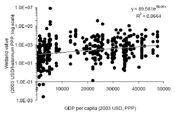
Exhibit 53 Wetland Value Plotted Against Total Population in 50km radius (Ghermandi et al. (2009))
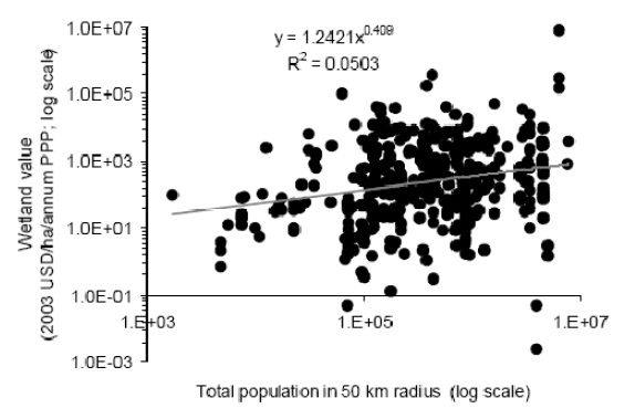
Exhibit 54 Wetland Value Plotted Against Wetland Size (Ghermandi et al. (2009))
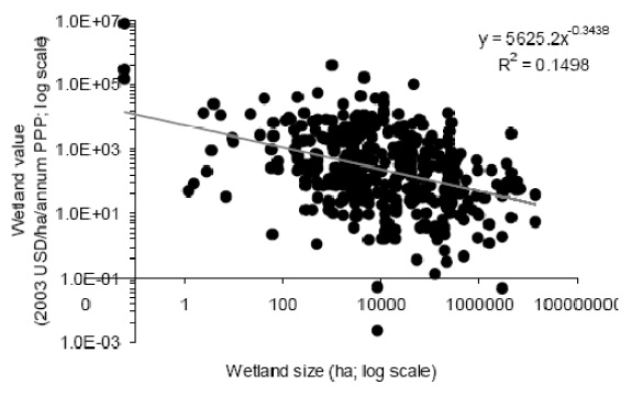
Exhibit 55 Wetland Value Plotted Against Wetland Abundance (Ghermandi et al. (2009))
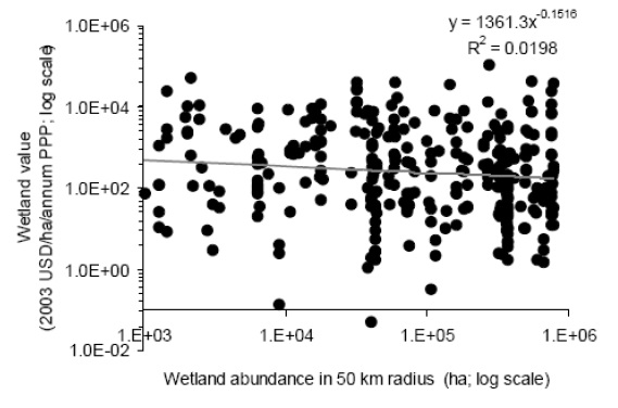
Appendix E Input Values and 30-year Trends of Costs and Benefits Conservation Authorities Contacts and Questions
This section summarizes the monetized results and provides the relevant input information for the uncertainty analysis. Specialized software was applied to develop the uncertainty analysis as described in Section 2 above. Exhibit 56 to Exhibit 61 following summarizes the input data for the uncertainty analysis and represents the low, middle and high input variables for the various habitat types. As noted above, the RiskTrigen triangular distribution function is attached to all the modeled variables. In addition to the inputs below, the discount rate is also modeled with uncertainty and ranging from 2% to 5%.
Exhibit 61, Exhibit 62 and Exhibit 63 graphically present the 30-year undiscounted stream of costs and benefits for both wetlands and stream systems for each of the three watersheds. These are presented in cumulative terms.
| Cost | Low Estimate | Middle Estimate | High Estimate | |
|---|---|---|---|---|
| Wetlands | Protection Costs | $2,109,931 | $2,699,748 | $3,289,565 |
| Wetlands | Restoration Costs | $3,192,864 | $4,257,152 | $5,321,440 |
| Wetlands | Total Wetland Costs | $5,302,795 | $6,956,900 | $8,611,005 |
| Stream Systems | Protection Costs | $664,667,620 | $850,471,062 | $1,036,274,505 |
| Stream Systems | River Restoration Costs | $16,310,890 | $21,747,853 | $27,184,816 |
| Stream Systems | Riparian Restoration Costs | $34,855,909 | $46,474,546 | $58,093,182 |
| Stream Systems | Upland Restoration Costs | $37,508,319 | $50,011,093 | $62,513,866 |
| Stream Systems | Total Stream Costs | $753,342,738 | $968,704,553 | $1,184,066,369 |
| Total Costs | $758,645,533 | $975,661,453 | $1,192,677,373 |
| Cost | Low Estimate | Middle Estimate | High Estimate | |
|---|---|---|---|---|
| Wetlands | Protection Costs | $1,013,635 | $1,607,901 | $2,202,167 |
| Wetlands | Restoration Costs | $1,064,830 | $1,419,773 | $1,774,716 |
| Wetlands | Total Wetland Costs | $2,078,465 | $3,027,674 | $3,976,883 |
| Stream Systems | Protection Costs | $927,730,557 | $1,471,633,372 | $2,015,536,188 |
| Stream Systems | River Restoration Costs | $17,768,379 | $23,691,172 | $29,613,965 |
| Stream Systems | Riparian Restoration Costs | $33,773,825 | $45,031,767 | $56,289,708 |
| Stream Systems | Upland Restoration Costs | $36,343,893 | $48,458,523 | $60,573,154 |
| Stream Systems | Total Stream Costs | $1,015,616,653 | $1,588,814,834 | $2,162,013,015 |
| Total Costs | $1,017,695,118 | $1,591,842,508 | $2,165,989,898 |
| Cost | Low Estimate | Middle Estimate | High Estimate | |
|---|---|---|---|---|
| Wetlands | Protection Costs | $4,991,426 | $6,655,234 | $8,319,043 |
| Wetlands | Restoration Costs | $16,866,038 | $22,488,051 | $28,110,064 |
| Wetlands | Total Wetland Costs | $21,857,464 | $29,143,285 | $36,429,106 |
| Stream Systems | Protection Costs | $62,465,286 | $83,287,047 | $104,108,809 |
| Stream Systems | River Restoration Costs | $757,291 | $1,009,721 | $1,262,152 |
| Stream Systems | Riparian Restoration Costs | $7,314,537 | $9,752,716 | $12,190,895 |
| Stream Systems | Upland Restoration Costs | $7,871,147 | $10,494,863 | $13,118,579 |
| Stream Systems | Total Stream Costs | $78,408,261 | $104,544,348 | $130,680,435 |
| Total Costs | $100,265,725 | $133,687,633 | $167,109,542 |
| Benefit | Low Estimate | Middle Estimate | High Estimate | |
|---|---|---|---|---|
| Wetlands | Annual Benefits Large Wetland | $102,785 | $204,785 | $306,784 |
| Wetlands | Annual Benefits Other Wetland | $4,592,214 | $9,986,539 | $15,380,863 |
| Wetlands | Total Wetland Benefit | $4,695,000 | $10,191,324 | $15,687,648 |
| Stream Systems | Annual Benefit Stream | $145,714,533 | $148,643,615 | $151,572,698 |
| Total Benefit | $150,409,532 | $158,834,939 | $167,260,346 |
| Benefit | Low Estimate | Middle Estimate | High Estimate | |
|---|---|---|---|---|
| Wetlands | Annual Benefits Other Wetland | $3,099,502 | $5,362,048 | $7,624,594 |
| Wetlands | Annual Benefits Open Shoreline Wetland | $908,745 | $965,448 | $1,022,151 |
| Wetlands | Annual Benefits Semi Protected Wetland | $177,316 | $193,808 | $210,299 |
| Wetlands | Total Wetland Benefit | $4,185,563 | $6,521,303 | $8,857,044 |
| Stream Systems | Annual Benefit Stream | $114,442,337 | $176,534,484 | $238,626,630 |
| Total Benefit | $118,627,900 | $183,055,787 | $247,483,674 |
| Benefit | Low Estimate | Middle Estimate | High Estimate | |
|---|---|---|---|---|
| Wetlands | Annual Benefits Large Wetland | $1,416,384 | $2,489,025 | $3,561,666 |
| Wetlands | Annual Benefits Other Wetland | $18,957,174 | $21,076,880 | $23,196,586 |
| Wetlands | Total Wetland Benefit | $20,373,558 | $23,565,905 | $26,758,252 |
| Stream Systems | Annual Benefit Stream | $47,431,410 | $51,473,336 | $55,515,261 |
| Total Benefit | $67,804,968 | $75,039,241 | $82,273,513 |
Exhibit 62 30-year Undiscounted Stream of Costs and Benefits for Credit River – 16 Mile Creek
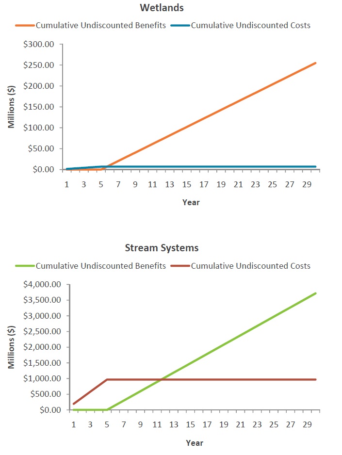
Exhibit 63 30-year Undiscounted Stream of Costs and Benefits for Toronto Region River
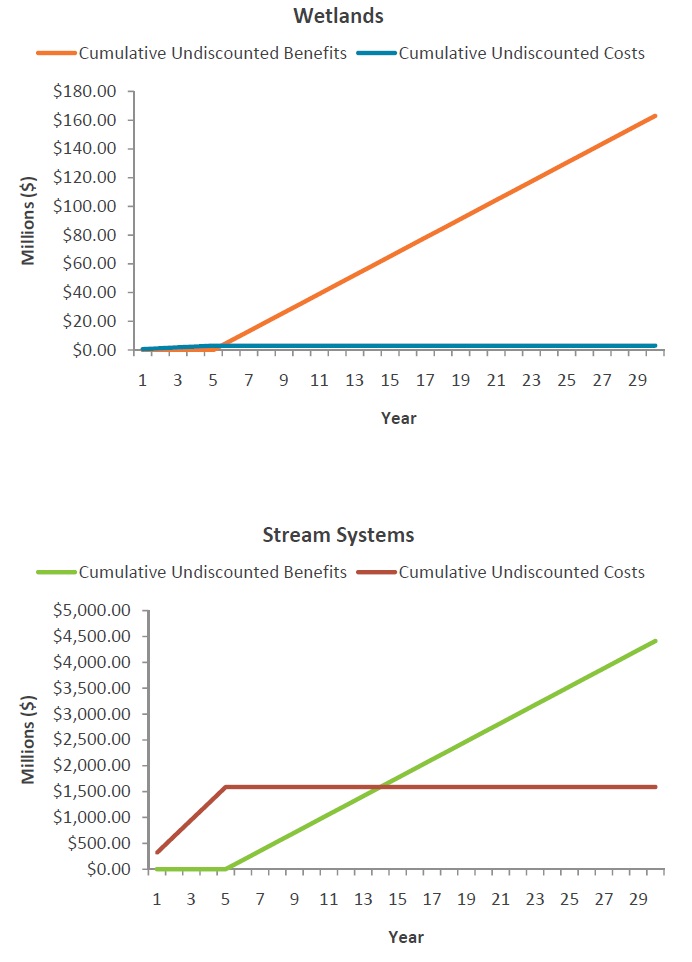
Exhibit 64 30-year Undiscounted Stream of Costs and Benefits for Prince Edward Bay
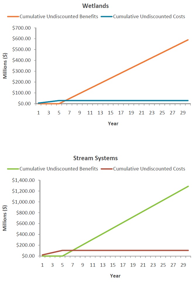
Appendix F Conservation Authorities Contacts and Questions
| Conservation Authority | Contact |
|---|---|
| Quinte Conservation | Tim Trustham |
| Bay of Quinte RAP | Anne Anderson |
| Toronto and Region Conservation Authority | Sonya Meek |
| Toronto and Region Conservation Authority | Dena Lewis |
| Credit Valley Conservation | Mike Puddister |
| Credit Valley Conservation | Kate Hayes |
| Conservation Ontario | Jo-Anne Rzadki |
Example Query Submitted to Conservation Authorities
Background:
As discussed, the study for the Ontario MOE undertakes a cost-benefit analysis of intervention strategies aimed at protecting and restoring habitats. We are using the Great Lakes Conservation Blueprint for Aquatic Biodiversity to identify our conservation goals for each watershed. The main habitat categories are Wetlands and Stream Systems, with consideration of Great Lakes Shoreline as well. The intervention strategies that we are looking at in detail are restoration and protection.
Restoration refers to active restoration of degraded habitat and protection refers to land securement. (For our purposes, securement is defined as the protection of habitat by purchasing lands or acquiring the title to lands through donations. The more traditional means of securing land for conservation includes government purchases of land to create or expand provincial parks, conservation reserves, or protected areas. Land can also be purchased by private actors and non-governmental organizations.)
With the help of the Conservation Authorities, we would like to determine the optimal mix between restoration and protection interventions needed to achieve the conservation goals.
Natural Cover, as defined in the Great Lakes Conservation Blueprint for Aquatic Biodiversity, ranges on a scale from 0% - 100%. All of the areas that were considered non-natural (cropland, urban areas, etc.) were classified to a value of 0% and all areas that were considered natural (i.e., lakes and wetlands) were classified to a value of 100%. The percentage of natural cover for the other habitats (e.g., stream and coastal) was then calculated on the scale 0% < X < 100%. (Aquatic Ecological Units (how the Blueprint is divided) that contained a large amount of Natural Cover were given priority in the Conservation Blueprint.)
Questions for Conservation Authorities (CA):
- Our study examines two intervention strategies to protect habitat: land purchase and restoration. A third category, “other”, will be identified but not analyzed (which could include stewardship, land easement, etc.). Is the X%/Y% allocation assigned in the table below for the two intervention strategies reasonable? In other words, within each habitat, is the level of active restoration reasonable versus what natural cover could be purchased/protected and left to regenerate on its own?
- Insert table with habitat and intervention allocation for relevant watershed (example provided)
Exhibit 66 Example of Information Request from Conservation Authorities Habitat Total area (ha) in WS 2HE Total area (ha) in all CL Area (ha) in BP Additional area (ha) to conserve Area (ha) to conserve already in NC Area (ha) needed not in NC Intervention * - Active Restoration Intervention * - Purchase / Protection Intervention - Other Shoreline 1283 141 177 35 35 0 30% 70% Headwaters 76170 1211 13376 12165 7817 4349 40% 60% Main Stem 160 20 48 28 28 0 40% 60% Large Wetlands 2873 2645 2872 227 227 0 40% 60% Stewardship Other Wetlands 12934 5287 6033 746 746 0 40% 60% Stewardship Other 12604 923 1533 610 551 60 * Assuming that Restoration includes Protection; and Purchase/Protection refers to the acquisition of land, which is left to regenerate on its own.
** The area (ha) for the Stream Systems (Headwaters, Middle Tributaries, Main Stem) include the stream itself and the riparian area (up to 300 m).
- If we are looking strictly at protection and restoration as intervention measures, is it reasonable to assume that any land under “Natural Cover” can just be protected? Or does the quality of the Natural Cover vary such that land considered as Natural Cover may still need to be restored? If this assumption is valid in your Conservation Authority area, would this assumption include wetlands? (e.g., a wetland would be 100% natural cover, but may need restoration as well as protection).
- What are the current habitat protection/restoration projects in the CA area? List and briefly describe (one – two sentences).
- What have been the most common stream / wetland / coastal restoration activities in the recent past: for agricultural lands; for urban lands; other lands? Would these same measures be applied moving forward (i.e., have they been successful?)?
- Can you share with us the costs of the recent (or planned) restoration (and protection) projects?
- Is there a different approach, different level of feasibility when working with municipal / provincial governments, private land-owners, etc..?
- Is it possible to estimate the percentage of streams in an urban area versus non-urban (e.g., 10% urban, 90% non-urban)? If so, what is your estimate?
Appendix G References
Amigues, J.P., Boulatoff. C., Desaigues, B., Gauthier, C., and Keith, J.E. (2002). The benefits and costs of riparian analysis habitat preservation: a willingness to accept/willingness to pay contingent valuation approach. Ecol Econ 43: 17–31
Austin, J., Anderson, S., Courant, P., Litan, R. (2007) “America’s North Coast: A Benefit-Cost Analysis of Program to Protect and Restore the Great Lakes.” pp. 86.
Boardman, A., M. Moore, A. Vining. (2009). Proposed Social Discount Rate(s) for Canada Based on Future Growth. PRI Project.
Brander, L.M., R.J.G.M. Florax and J.E. Vermaat (2006). The empirics of wetland valuation: a comprehensive summary and a meta-analysis of the literature. Environmental and Resource Economics 33:223–50.
Brander, Luke M., Ghermandi, Andrea, Kuik, Onno, Markandya, Anil, Nunes, Paulo A. L. D., Schaafsma, Marije and Wagtendonk, Alfred (2010). Scaling Up Ecosystem Services Values: Methodology, Applicability and a Case Study. FEEM Working Paper No. 41.2010.
Breunig, K. (2003). Accounting for the Economic Value of Ecosystem Services in Massachusetts. Losing Ground: At What Cost? 3rd Edition, Boston: MassAudubon
Brouwer, R., I.J. Langford, T.C. Bateman, T.C. Crowards and R.K. Turner (1999). A meta-analysis of wetland contingent valuation studies. Regional Environmental Change 1:47–57.
CEC (Commission for Environmental Cooperation) (2006). Factual Record Ontario Logging Submission (SEM-02-001) and Ontario Logging II Submission (SEM-04-006). 272 pp.
City of Toronto (2003). Wet Weather Flow Master Plan: List of CSO/Stormwater Control Alternatives. pp.275
Credit Valley Conservation, Credit River Water Management Study Update, May 2007.
Crombie, D. (1992). Regeneration: Toronto’s Waterfront and the Sustainable City: Final Report. Royal Commission on the Future of the Toronto Waterfront. pp. 530.
David Suzuki Foundation (2008). Ontario’s Wealth, Canada’s Future: Appreciating the Value of the Greenbelt’s Eco-Services.
Dodds, R. (2010). Determining the Economic Impact of Beaches: Lake Huron Shoreline from Sarnia to Tobermory. Ryerson University, Ted Rogers School of Hospitality and Tourism Management. pp. 17.
Ducks Unlimited Canada (2010). Conservation Easements: Partnerships for Conservation.
Environment Canada, Ontario Ministry of Natural Resources, and Ontario Ministry of Environment. (1998) A framework for guiding habitat rehabilitation in Great Lakes Areas of Concern. Canada-Ontario Remedial Action Plan Steering Committee. 75 pp.
Environment Canada (2010). Rehabilitation and Securement. Last modified 02-26-2010.
EPA (2000). Economic, Environmental and Benefits Analysis of the Proposed Metal Products and Machinery Rule. Office of Science and Technology. EPA-821-B-00-008.
Freeman, A.M. III. (1979). “The Benefits of Environmental Improvement: Theory and Practice” The Johns Hopkins University Press, Md., for Resources for the Future.
Ghermandi, Andrea, Jeroen C.J.M. van den Bergh, Luke M. Brander, Henri L.F. de Groot, Paulo A.L.D. Nunes (2009). The Values of Natural and Constructed Wetlands: A Meta-Analysis. Tinbergen Institute Discussion Papers 09-080/3, Tinbergen Institute.
Hasset, B., Palmer, M., Bernhardt, E., Smith, S., Carr, J., and Hart, D. (2005). Restoring watersheds project by project: trends in Chesapeake Bay tributary restoration. Frontiers in Ecology and the Environment, 3.5: 259–267.
Hayes, L. (2010). Personal Communication. Project Leader, Restoration and Stewardship. Credit Valley Conservation. Email: khayes@creditvalleyca.ca
HM Treasury (2003). Appraisal and Evaluation in Central Government (The Green Book). London: HMSO.
Holmes, T.P., Bergstrom, J.C., Huszar, E., Kask, S.B. & Orr, F. (2004). Contingent valuation, net marginal benefits, and the scale of riparian ecosystem restoration. Ecological Economics, 49.1: 19-30.
International Lake Ontario-St. Lawrence River Study Board (2006). Valuing Wetland benefits compared with Economic Benefits and Losses. Report to the International Joint Commission.
Jacobsen, J.B., Hanley, N. (2009). Are there income effects on global willingness to pay for biodiversity conservation? Environmental and Resource Economics, 43.2: 137-160.
Kennedy, M. and J. Wilson (2009). Estimating the Value of Natural Capital in the Credit River Watershed. Pembina Institute.
Lake Ontario Biodiversity Strategy Working Group in co-operation with the U.S.–Canada Lake Ontario Lake wide Management Plan (2009), The Beautiful Lake: A Bi-national Biodiversity Conservation Strategy for Lake Ontario
Lawrence, P.L. (1995). Development of Great Lakes shoreline management plans by Ontario conservation authorities. Coastal and Ocean Management, 26.3: 205-223.
Lawrence, P.L. (1998). Ontario-great lakes shoreline management: An update. Coastal and Ocean Management, 26.2: 93-104.
Lebegue, D., Baumstark, L. and Hartzmanm P. (2005) Revision Du Taux D’Actualisation Des Investissements Publics. Rapport du Groupe d’Experts Preside par Daniel Lebegue, Commissariat General du Plan.
Lewis, D. (2010). Personal Communication. Manager of Terrestrial and Aquatic Ecology. Toronto and Region Conservation Authority. Email: dlewis@trca.on.ca
Loomis, J., et al. (2000). Measuring the total economic value of restoring ecosystem services in an impaired river basin: Results from a contingent valuation survey. Ecological Economics, 33(1), 103-117.
Moore, M.A., A. Boardman and D. Greenberg (2004). Just Give Me a Number!: Practical Values for the Social Discount Rate. Journal of Policy Analysis and Management 23(4): 789-812.
Nature Conservancy Canada (2010). Gifts of Land: What is a Conservation Agreement?
Nature Conservancy of Canada and the Ontario Ministry of Natural Resources. Great Lakes Conservation Blueprint for Aquatic Biodiversity (2005).
NOAA (National Oceanic and Atmospheric Administration) (2010). Shoreline Management Resources.
Nolan, J. (2004). Ontario Stream Restoration - Planning and Projects. Division of the Environment - University of Toronto: Toronto, ON. Published 05-05-2004, revised 09-26-2008.
Olewiler, N. (2004). The Value of Natural Capital in Settled Areas of Canada, Ducks Unlimited Canada and the Nature Conservancy of Canada.
OMF (Ontario Ministry of Finance) (2010). Ontario’s Long Term Report on the Economy. 167 pp. OMNR (Ontario Ministry of Natural Resources) (2005). Ontario’s Biodiversity Strategy. 52 pp.
OMNR. Wetland Restoration. Available at: Ministry of Natural Resources - Wetland Restoration
Pascual, Unai and Roldan Muradian, (2010). The economics of valuain ecosystem services and biodiversity. Chapter 5 of the Ecological and Economic Foundation Report.
Roni, P., Hanson, K., Beechie, T., Pess, G., Pollock, M. and Bartley, M.D. (2005). Habitat rehabilitation for inland fisheries. Global review of effectiveness and guidance for rehabilitation of freshwater ecosystems. FAO Fisheries Technical Paper. No. 484. Rome, FAO. Pp. 116.
Schollen, M. (2010). Personal Communication. Principal. Schollen & Company Inc. marks@schollenandcompany.com
Schuyt, Kirsten and Luke Brander (2004). The economic values of the world’s wetlands. WWF.
Sverrisson, D. (2008). Estimation of the Passive Use Value Associated with Future Expansion of Provincial Parks and Protected Areas in Southern Ontario. MSc Thesis Agricultural and Rural Economics. University of Alberta.
Tejani, R. and Muir, T. (2003). Monetary benefits of the Hamilton-Halton Watershed Stewardship Program (1994-2002): Cost Savings and Economic Benefits. Report for Great Lakes Sustainability Fund.
Thayer, G.W., McTigue, T.A., Bellmer, R.J., Burrows, F.M., Merkey, D.H., Nickens, A.D., et al. (2003). Science-based restoration monitoring of coastal habitats. National Oceanic and Atmospheric Administration Coastal Ocean Program, Decision Analysis Series, 23.1.
Toronto and Region Conservation Authority, Humber River Watershed Plan: Pathways to a Healthy Humber, June 2008.
Toronto and Region Conservation Authority (TRCA). 2007. Terrestrial Natural Heritage System Strategy.
Treasury Board of Canada Secretariat (TBS) (2007). Social Discount Rates for Canada (Draft.) PRI Project.
Troy, A. and Bagstad, K. (2009). Estimating Ecosystem Services in Southern Ontario. Report for Ontario Ministry of Natural Resources.
USACE (US Army Corps of Engineers). Great Lakes Habitat Initiative Final Report and Implementation Plan. 125 pp. 2008
U.S. Army Corps of Engineers (2008). Great Lakes Habitat Initiative Final Report and Implementation Plan.
Wichert, G.A., K.E. Brodribb, B.L. Henson, and C. Phair, Great Lakes Conservation Blueprint for Aquatic Biodiversity, Volume 1, Nature Conservancy Canada, Natural Heritage Information Centre, Ontario Ministry of Natural Resources, 2005.
Wilson, Sara J. (2008). “Lake Simcoe Basin’s Natural Capital: The Value of the Watershed’s Ecosystem Services”. Prepared for Friends of the Greenbelt Foundation Occasional Paper Series.
Woodward, R.T. and Wui, Y.S. (2001). "The economic value of wetland services: A meta- analysis" Ecological Economics 37:257-270.
222 Somerset Street West, Suite 300
Ottawa, Ontario, Canada K2P 2G3
info@marbek.ca
www.marbek.ca
Project ID: 10033