Summer profundal index netting manual
Manual of Instructions for Summer Profundal Index Netting (SPIN): A Lake Trout Assessment Tool
Science and Information Resources Division
Ontario Ministry of Natural Resources
Version 2009.1
This Manual should be cited as follows: Sandstrom, S. J. and N. Lester. 2009. Summer Profundal Index Netting Protocol; a Lake Trout Assessment Tool. Ontario Ministry of Natural Resources. Peterborough, Ontario. Version 2009.1. 22 p. + appendices.
Accessibility
We are committed to providing accessible customer service.
If you need alternative accessible formats or communications supports, contact us.
If you have questions about summer profundal index netting, contact Blair Wasylenko.
1.0 Introduction
Lake trout (Salvelinus namaycush) are known to inhabit a wide range of lake sizes which often require a different approach and intensity of sampling. Across lakes this species is known to exhibit several life history strategies resulting in divergence of possible adult size spectra, and within a lake occupies neither a predictable nor constant distribution. Being a highly prized catch of fishermen and occupying deep clear lakes, ideal for recreation, populations are often in a degraded state, real or perceived, calling for a cautious sampling approach. Faced with this level of variability it would be difficult to develop a “one method fits all” approach to lake trout assessment in Ontario. Rather, what is needed is a method with some degree of flexibility so that it can be molded, while still maintaining comparability, to suit the specific conditions of the intended lake and population.
The Summer Profundal Indexing Netting (SPIN) Protocol outlined in this report is an adaptable methodology that can be used to assess both small bodied and large bodied lake trout population in a wide range of lake sizes. It was developed as a rapid assessment method requiring less than a week to complete most lake surveys, offering a low mortality option for sensitive populations and providing a lengthy window of operation so many lakes could be surveyed by a single crew in a season.
The SPIN methodology is guided by two basic objectives utilizing one gear type applied over a series of depth criteria and time options.
1.1 Program objectives
1.1.1 Lake trout density estimation
The primary objective of SPIN is to estimate the density of harvestable sized lake trout in a lake. To do this the method uses gillnets which are designed, through a careful selection of mesh sizes, to capture lake trout greater than 300mm fork length. This size was chosen as the minimum for a number of reasons:
- Anglers tend to harvest fish larger than this size, hence, consequences of exploitation should be detectable.
- In order for the method to be able to provide an estimation of density it must be calibrated in populations of known abundance. This is typically done via mark–recapture procedures involving adult fish (>300 mm in Ontario) tagged on the spawning shoals. Thus, although there would be potential to capture smaller fish by including smaller mesh sizes, it would be without ability to translate into a usable density.
- This limit on the minimum size of fish selected improves the low mortality feature of the index by avoiding very small lake trout which appear to be less able to regulate swim bladder volume on ascent, and thus, exhibit a disproportionately greater sampling mortality
- Avoiding mesh that would select for fish of forage size to a lake trout minimizes the possibility that catchability of these isn’t artificially elevated by what would functionally be described as ‘baiting’ the net.
Density estimates are obtained by calculating the selectivity corrected area weighted average arithmetic catch per 64m net. The calculation of relative density does not require a large biological sample and is guided by the appropriate number of samples (net sets) being taken from each stratum. The SPIN(L2) (aka daytime) method outlined herein has been calibrated to density, and can be used to estimate number of lake trout in a lake. The SPIN(L18) (aka overnight) is optional and is used primarily to assist with addressing the second objective (discussed below) in low density lakes.
Although this method can provide an estimate of the number or density of fish in the lake, this alone often does not provide us with enough information to determine how many fish should be in a particular lake (i.e., status: is a management action warranted?). To derive an understanding of this requires additional information:
- physical/chemical attributes of the lake
- biological attributes of the species
- biological attributes of lake (species complex)
The remaining objective of the SPIN protocol is directed at addressing the additional biological information needed for status determination.
1.1.2 Lake trout biological indicators
The second objective is the attainment of a representative sample of adult lake trout across the range of lake depth and area. This would be used to evaluate the biological integrity of the population and to monitor for effects of exploitation on life history characteristics. Currently the required sample is in the order of 75 lake trout; however, this should not be considered a maximum if a larger sample is possible within the timelines of the project, and can be supported by the available population biomass. Similar interpretations may be possible from a smaller sample, but sample sizes less than 30 fish will likely be insufficient to produce reliable results.
In isolation, the biological objective is not contingent on a specific sample size (i.e., number of net sets), but sampling should be approximately representative of area/depth of lake. Any number of sets, of different duration, over a broad period of time could be used to obtain the biological objective for a particular lake in a given season. However, if care is taken to ensure that a sufficient number of similar duration sets are used, as specified in this manual, then a comparable density estimate may also be attainable from the information.
The biological sample can either be live or dead sampled, but the latter has advantages as maturity and sex specific growth parameters can be determined. Diet information, from a dead sample, can indirectly yield important insights into trophic status, movement and behavior of the population.
This data may be extremely useful in categorizing the catchability of the population using this methodology and may improve interpretations made from it.
Key diagnostic parameters to evaluate include:
- Size and / or age at maturity
- Estimate of survival (length or age based)
- Growth parameters such as K, to and Linf (if otolith ages available)
2.0 Field methodology
Biologists who intend on doing a SPIN project are advised to first contact the Aquatics Science Unit (ASU) of the Ministry of Natural Resources (see contact information at front of report). Staff here are prepared to provide support in project design, equipment use, data entry and subsequent data analyses should this be required.
If a bathymetric map is not available, it is strongly recommended that a bathymetric survey (collection of xyz coordinates) be conducted to create a hydrographic map of the intended lake prior to the start of the project. This will not only assist in sample size determination and final calculation of the area weighted density estimate, but will greatly simplify the site selection process. An example of a SPIN bathymetric sampling map is provided in Appendix I.
2.1 Summary
Criteria
Season
Surface water greater than 18°C or 4–6 weeks of peak summer temp for northern systems
Set Durations
SPIN(L2) two hour (min); two hours twenty minutes (max) SPIN(L18) eighteen hours (min); twenty hours (max)
Gear Length
64m (8 mesh sizes x 8 m panels)
Mesh Series
2.25, 2.50, 2.75, 3.0, 3.5, 4.0, 4.5, 5.0 (stretch inch)
Set Orientation
Random
Depth
7 Strata (2–10m, 10–20m, 20–30m, 30–40m, 40–60m, 60–80m, 80+m)
Spatial Stratification
Effort equally distributed over entire lake
No. Samples per Lake
No. of Sets SPIN(L2) = 0.0184(Area >10m, ha) + 24 (max. 140)
Minimum of three sets in non–core stratum and five in core stratum (10–40m)
No. Sets per Day
6, 9 or 12 sets
Target Biological Sample
n = 75+ lake trout
Overall Target CUE
Relative Standard Error = 0.15
2.2 Project timing
Netting should be conducted once surface water temperature has warmed to greater than 18 degrees Celsius, and concluded when temperature drops below 18 degrees Celsius. This should ensure that most lake trout are in the hypoliminon (typically greater than nine meters in most Ontario lakes) where sampling is concentrated. In more northern or Arctic lakes where surface temperatures may not reach 18 degrees Celsius, sampling should occur during the four to six weeks of peak summer water temperatures.
2.3 Gear type
2.3.1 Mesh size
Nets are 64 m long (8 mesh sizes x 8m panels) by 1.8 m high and have the following stretch mesh sizes; 57mm (2.25”), 64mm (2.50”), 70mm (2.75”), 76mm (3.00”), 89mm (3.50”), 102mm (4.0”), 114mm (4.5”) and 127mm (5.0”). All panels in the gang are sewn together and hung on the half (2m of mesh to 1m of lead line). All mesh sizes use double knotted construction. The diameter of monofilament (mm), in order of increasing mesh size, is as follows; 0.23, 0.23, 0.23, 0.28, 0.28, 0.33, 0.33, 0.33.
| Stretch measure (in) | 2.26 | 2.60 | 2.76 | 3.00 | 3.50 | 4.00 | 4.50 | 5.00 |
|---|---|---|---|---|---|---|---|---|
| Stretch measure (mm) | 57 | 64 | 70 | 76 | 89 | 102 | 114 | 127 |
| Mono diameter (mm) | 0.23 | 0.23 | 0.23 | 0.28 | 0.28 | 0.33 | 0.33 | 0.33 |
| Series Order 1 | 7 | 3 | 6 | 2 | 6 | 1 | 4 | 8 |
| Series Order 2 | 6 | 2 | 4 | 8 | 7 | 5 | 1 | 3 |
| Series Order 3 | 6 | 8 | 2 | 5 | 1 | 4 | 7 | 3 |
| Panel length (m) | 8.0 | 8.0 | 8.0 | 8.0 | 8.0 | 8.0 | 8.0 | 8.0 |
| Panel length (ft) | 26.2 | 26.2 | 26.2 | 26.2 | 26.2 | 26.2 | 26.2 | 26.2 |
| Panel height (m) | 1.8 | 1.8 | 1.8 | 1.8 | 1.8 | 1.8 | 1.8 | 1.8 |
| Panel height (ft) | 5.9 | 5.9 | 6.9 | 5.9 | 6.9 | 5.9 | 6.9 | 6.9 |
2.3.2 Mesh series
One of three different random series of meshes are fished simultaneously. Several random configurations are employed to minimize the potential for competing influence of certain neighboring mesh panels. Also, as the geometry of the end panel is different than those in the middle of the gang when the net is set, varying the end mesh panels will reduce the affect this may have on CUE.
2.3.3 Composition
Gangs are constructed using Number 30 lead line (15lbs/300ft) and 0.5 inch (13mm) braided float line. All nets have a standardized spanner (often incorrectly referred to as bridles) length (4 m) to ensure a more consistent set among offices or agencies. Spanner length can adversely affect net profile, particularly in the end Goop© panels, if it is too short. Mesh labels (collars)

The end of each panel is clearly labeled with its corresponding mesh size using a labeled metal bird band and the division identified with a distinctive colour flash. To prevent the band from snagging in the net, the seam is sealed using a waterproof adhesive like marine Goop©.
Prices for SPIN gangs will vary between years and builders; it is recommended that the buyer shop around for the best price. Below is a list of builders that have the specified material in stock and are able to build SPIN nets.
| SPIN Builders | Address | City | Province | PC | Phone # |
|---|---|---|---|---|---|
| Lakefish Net and Twine | 547 King Edward St. | Winnipeg | MB | R3H 0N9 | |
| Johnson Net and Twine | 859 Talbot road East | Wheatley | ON | P0P 2P0 | |
| Les Industries Fipec Inc. | 235 La Grande–Allee Est | Grande Riviere | QC | G0C 1V0 |
2.4 Set orientation
Nets are set on bottom (benthic) and orientation is random at all start depths, some moderate deviation from the random criteria can be made to ensure the net does not leave the stratum should the specific site bathymetry warrant. Prevailing weather conditions will dictate the degree of randomness possible. Nets set in depths less than five meters should be set perpendicular to shore.
2.5 Depth strata
Individual sets should not be allowed to span more than one stratum. Stratum of less than 20 hectares should be combined with the adjacent shallower stratum
Stratum 1 = 2 m – 10 m
Stratum 2 = 10 m – 20 m (Core)
Stratum 3 = 20 m – 30 m (Core)
Stratum 4 = 30 m – 40 m (Core)
Stratum 5 = 40 m – 60 m
Stratum 6 = 60 m – 80 m
Stratum 7 = 80+ m
2.6 Duration of set
To impart some flexibility in application of the method, the SPIN protocol has the option of utilizing two different set durations.
2.6.1 Two hour set duration (+ 20 minutes) – SPIN(L2) (aka daytime sets)
This duration is best suited for projects where live sampling is required, or, where setting nets overnight is deemed socially and/or biologically unacceptable. Also in very high density lakes (either lake trout or other cold water species like whitefish) the shorter set duration is advised as net saturation may negatively influence catch rates. Saturation limits for this gear have been modeled at approximately 26 kg per net. Results from lakes were catches (all species) exceed this should be treated with caution.
- Daily sampling intensity ranges between six to12 sets a day, set and retrieved on 20–40 minute intervals
- Fish can be either live sampled or dead sampled
- Lake trout survival is approximately 70% on average
- Period of sampling for daytime sets is from 8:00 am to 17:00 pm (+/- one hour)
Calibration of index CUE with density has only be completed for the SPIN(L2) method.
2.6.2 Eighteen hour set duration (± 120 minutes) – SPIN(L18) (aka overnight sets)
As the majority of catch is killed in these sets, this approach is more suited for lakes where concerns regarding sampling mortality are minimal. It has been observed that catchability of small bodied lake trout is approximately four times lower than that of large body lake trout (see Section 3.3 for details) resulting in typically low CUEs and corresponding small project sample sizes when using the SPIN(L2) method. The longer duration is advised in these systems, if mortality isn’t an issue, as temporal changes in density may be more easily detected statistically and sample sizes more adequate for examination of life history parameters. This duration is also best suited for very large lakes where travel time to and from the netting location prohibit sampling with short duration sets. It also may be a better option for lakes with high water clarity (i.e., >7m Secchi reading) where net detection and avoidance may be an issue. This is also likely the best method to obtain the required biological samples in the shortest period of time, as daily catch rates are typically higher (roughly 4–6 times higher than two hour duration).
- Four or six sets a day, retrieved in the morning and reset at the end of the day
- Lake trout survival is approximately 30% in limited trials of this set duration
- Period of sampling for overnight sets spans the hours of 14:00 and 16:00 (set) and 8:00 and 10:00 (lift), in a way that soak time approximates 18 to 20 hours.
The SPIN(L2) and the SPIN(L18) can also be used concurrently in lake, such as those with moderate mortality issues and/or where a sufficient biological sample can not be attained within the time constraints of the project using just two hour sets. SPIN(L18) sets can also be incorporated into the later stages of a SPIN(L2) project to increase the number of biological samples, while still permitting the determination of a relative density estimate using the two hour sets.
2.7 Number of samples
Suggested minimum sample size is dependent on the area (ha) of habitat >10m in the lake, rather than the total lake size, and the two vary in a linear fashion.
2.7.1 SPIN(L2) (two hour sets):
No. of Sets = 0.0184(>10m Area, ha) + 24 (maximum of 140 sets)
2.7.2 SPIN(L18) (18 hour sets):
No. of Sets = 0.008(>10m Area, ha) + 6 (maximum of 60 sets)
Formulas provide a rough approximation as to the required effort for a lake of a given size; however, if funding and time permits it is advantageous to maximize the number of sets in order to minimize error associated with the estimate of density (CUE). It is suggested that attainment of a relative standard error (RSE) of 0.15 ± .05 be the level desired for the project. The relative standard error (RSE) is a measure of an estimate’s reliability. The RSE is obtained by dividing the standard error of the estimate (SE(r)) by the estimate itself (r). It is useful to track the daily changes in RSE (as sample size increases) during the course of a project to permit the exploration (i.e., extrapolation) of whether further sampling will be analytically advantageous.
2.8 Spatial allocation of effort
2.8.1 Allocation to lake
Effort should be made to allocate sets equally to all regions of the lake. Dividing the lake up into a number of approximately equal–sized sectors and allocating the required samples similarly among these is the best approach. Selection of the required sample sites within lake or sector can be done by random grid selection, or if there is no real or preconceived knowledge of lake trout distribution, simply by visually ensuring even coverage. In large lakes where travel time may prevent the full spatial extent of the lake or sector to be sampled daily, grouping sites into manageable clusters is an acceptable compromise; however, nets should not be set simultaneously within 250 m of each other. In very small lakes where this interval may be difficult to achieve, neighboring sets should be at congruent angles to one another.
2.8.2 Allocation to stratum
Allocation of effort (# samples per day per stratum) depends on a number of factors:
- Set duration used (two eighteen hours).
- Number of full strata in lake
- Relative area of each stratum
- Catch success in each stratum
2.8.2.1 Two hour sets – SPIN(L2)
The number of daily sets (samples) possible will depend on the average CUE per net of all species combined. In lakes with high abundance of non–target species (e.g., herring, whitefish etc.) the maximum number of nets that can be set and processed in a day will be between six to nine sets. In lakes with ‘clean’ (i.e., lake trout only) catches, nine to twelve sets a day are likely possible.
As a general rule, a minimum of three daytime sets for each available non–core strata (1, 5–7) and a minimum of five sets in core strata (2–4) should be completed, regardless of lake size. If lake trout are not observed in any stratum after this minimum allocation, then the stratum can be dropped from further sampling to more efficiently allocate any remaining effort. The amount of sets allocated to lake trout producing stratum in subsequent days will depend on the proportion of sampled area (>10m in depth, ha) that the stratum occupies, and the relative density of lake trout within the stratum as determined from the initial minimum sample.
Number of Samples in Stratum A on Day i would be calculated as follows:

Where:
CUEA = Average CUE of Stratum A to day i (minimum value is 0.2)
AreaA = Area of Stratum A (ha)
DSS = Daily Sample Size (typically 9 sets)
The logic behind this approach is to balance the objectives of conducting both an area weighted sampling approach (i.e., larger strata get sampled more), and the requirement to obtain a representative biological sample. Strata with higher densities of lake trout get sampled somewhat more than others with lower densities, and this may not be in direct proportion to area. Variance typically increases with catch rates (CUE), thus, the optimal design should favor the strata where abundance is observed to be higher in attempt to reduce the variance and improve statistical interpretations. The result is an improved understanding of density in those strata where lake trout tend to concentrate, with the added benefit of obtaining a greater number of biological samples then would have been expected with a simple proportion of area sampling approach.
2.8.2.2 Sets – SPIN(L18)
The stratum sample sizes for the overnight method are considerably reduced from those required by SPIN(L2) projects, with small sample size varying the number of sets per stratum could potentially result in some having very few sets from which to draw conclusions about relative density. To prevent this, an equal allocation of daily samples to each stratum is recommended. Area weighting the final lake–wide mean catch would be calculated mathematically using the stratum proportions upon completion of the project. At least two overnight sets per stratum should be completed as a bare minimum, and core stratum should receive double this minimum. Also, as in the SPIN(L2) method, if lake trout are not observed after two or more sets in any particular stratum, then that stratum could be dropped from further sampling to more efficiently allocate the remaining effort. It is important to keep in mind that the SPIN(L18) is not calibrated with density (no. fish per hectare) and there are no studies planned to address this. Users of this set duration would be relying on CUE and changes in this as relative measures of density.
2.9 Setting nets
Established procedures should be followed for attaining permission to conduct a survey on the intended lake. Pertinent management agency/groups should be notified well in advance of work and written permission received prior to conducting any fieldwork.
Proper safety protocols should be developed prior to the field season with the appropriate manager’s input. These should be carefully reviewed with crew prior to work and revisited periodically during the program. Working in exposed boats during the height of summer can expose crews to heat related injuries. Sunscreen, sunglasses, hat, life jacket and water bottle should be part of every crew member’s personal onboard equipment. Appendix II contains a list of equipment that should be assembled to conduct a survey.
Dissolved oxygen and temperature profiles should be completed prior to the start of the project and areas/depths of <3 mg/l should receive the minimum number of sets (e.g., n=3 for SPIN(L2)) but then omitted from the survey if these do not indicate the presence of lake trout.
Nets should be neatly packed/loaded into fish tubs prior to heading out onto the water, or before setting a net. This is most easily accomplished by two people feeding the net into the bin/tub, keeping the lead line on one side and float line on the other. Tubs and the bow of boats should be checked for snags/burrs ahead of time and these removed so that nets flow smoothly out and aren’t inadvertently damaged during setting and pulling. A flat file should be included in the sampling kit for grinding down burrs which may occur from time to time from anchors knocking against the gunnels. Covering exposed rivets with a small flat spot of clear marine Goop (available at Canadian Tire) in areas where the net may contact the boat as it is set or retrieved will be helpful. Using duct or other types of tape is not advised, other than for a quick fix, as tape will often begin to detach over time and the lifted edges will themselves become a source of snagging.
It is important that the net remain fully within the stratum, it is a good practice that prior to the net being set, an initial pass of the intended location is made while viewing the area on the depth sounder (i.e., for 64 m or 128 m if two nets are joined), to ensure the net will fit fully within the depth stratum.
Net is deployed by first throwing out a float along with the rope making sure that there is enough line to reach bottom with some to spare, this will prevent the net from being lifted off the bottom by wave action. Clip or tie the end of this rope to the anchor and then to the first spanner, drop overboard and start paying out the net as the boat begins to back up very slowly. Periodically spread the float and lead line apart to check that they aren’t twisted. Setter(s) should indicate to the driver (or recorder) when the middle of the net is reached so that UTM coordinates can be recorded or marked. The driver should provide a depth to the setter(s) as the end of the net is reached so the appropriate amount of rope is used for the second float. Clip or tie the end spanner to the anchor and fasten the rope to this and drop overboard. Pay out all the rope quickly while the boat maintains position, once all the rope is out, the boat should continue reversing in a straight line. Holding onto the rope near the float, tighten the set until snug, not tight. Ensure that both floats are bobbing loosely on the surface. It is highly advised that two floats be used on each set, one per end, as it is inevitable that during the course of a project a float line will become detached or float sunk by accidental use insufficient line. A new dry net may take a few minutes to sink while the braided float line fills with water for the first time, crew should remain until this has submerged enough not to be a hazard to navigation.
Assembling a selection of rope of varying lengths, labelled at each end with the dimension, and assigned to appropriately labelled tubs/pails, make sorting and setting much easier. A series that has been shown to work well is as follows: 4 x 6m, 4 x 12m, 3 x 22m, 2 x 32m, 2 x 42m (and 2 x 62m if lake depth warrant). Used in combination, they can cover, without too much excess (and extra pulling), most of the required depths. A slip sheet bend knot, used for joining two ends or attaching anchors/floats is a very useful knot to have in one’s repertoire for this purpose. Sinking rope will reduce the possibility of any excess floating at the surface becoming a navigational hazard. Braided 3⁄8” nylon “yacht” rope has been found to work extremely well, it sinks, does not tangle unduly, lies nicely in pails and the larger diameter provides for better grip when pulling.
Slip Sheet Bend

All floats should be clearly marked with agency name and contact number and should include a caution that it is attached to scientific equipment and lifting and/or removal is prohibited. Effort should be made to advise the public, who are in the general area where work is being conducted, as to the nature. This especially pertains to anglers working the area with downriggers which may snag on the gear if they unknowingly troll near the marker float(s). Yellow has been found to be the best colour for detecting markers from a distance and during rough weather.
An image of a message from the Government of Ontario, reproduced as text below:
An important consideration to setting the nets correctly is anchor weight. Using too heavy an anchor will adversely affect the way the net is set and possibly unnecessarily fatigue the crew. In addition, heavy anchors can place excessive tension on the net which could negatively affect catchability of the gear. It is advised that anchors not exceed two kilograms in mass, often only half this will be sufficient (e.g., 5 or 6 links of 10mm grade 70 chain).
If the wind is strong, it is acceptable to set with it even if this deviates from the random approached stated herein. Often this will not require the motor and the driver can be freed to help with setting. A neatly pack net is required for this approach as there won’t be time to work out a tangle once the net starts going out.
Ensure the net is set in a straight line, it is not possible to straighten a net once more than 50% of it is deployed. An overly arced net will have to be retrieved into the boat before being reset straight. The primary cause of a ‘bent’ set is an incorrectly packed net, pausing during setting to untangle a net on a windy day will often have this result.
If possible, sampling days should occur on alternating days (e.g. Mon Wed Fri) to minimize weather influences. Spreading sampling effort over several weeks is recommended to further reduce this possibility. This approach is obviously better suited for the two hour daytime method.
For each of the sample days, nets should be set in all of the available strata as equally as possible (ie. do not set all nine sets in one strata, unless there is only one stratum), and each stratum should be fished one or more times in the morning and one or more times in the afternoon.
A particular stratum’s effort should be allocated ‘across’ the stratum. To do this, half of the allocation should target the shallower half and the remainder the deeper half of a stratum (e.g. shallow = 20-25 & deeper = 25-30m). Nets are allowed to freely cross over between the two sub–strata.
Careful attention should be taken that entire lake is proportionally and spatially sampled by the completion of the project.
For larger lakes, or lakes where individual net CUE would not hinder additional daily sets being made (i.e. low daily catch all species), it is suggested that two or more gangs of nets can be strapped together (i.e., joining them at the apex of the spanner – fishing more than one net per site). The sample CUE would be the average of the individual net CUEs. This approach would provide a more accurate lake wide CUE estimate (i.e., fewer zeros = lower RSE), and would double the number of biological samples collected by the project. The ability to fish paired sets will depend on lake size, weather, amount of catch, and crew size/ability.
2.10 Retreiving nets
Approach the downwind float and retrieve into the boat. A boat hook is a useful item to include in the list of onboard equipment. Double check depths and coordinates before lifting the first anchor to make sure you are pulling the right net.
Pull in the rope, depositing it directly into the appropriate labelled pail or tub. This will ensure that it goes back out tangle free on the next set and doesn’t interfere with current retrieval.
Pulling in the net, especially a double gang, should be done by two people, one pulling in the lead line while the other pulls the float line. When a fish is reached, one can work to remove this while the other continues pulling in both lines. If weather is rough, then often the driver must maintain the helm and control the boat as the net comes in, thus, a three person crew is recommended for most projects. The exception is in very small lakes where conditions likely won’t prevent the driver from participating in the physical aspects of lifting the net.
Although, recording catch by mesh is optional for District and partnership SPIN projects, all projects conducted by ASU offices must record this information in order to develop and refine the selectivity correction necessary for catch interpretation. It is important that care is taken in recording mesh size, because the two labels lie side by side the label from the proceeding panel can often be mistaken for the correct one (see picture in section 2.3.3). Adjoining panels often differ considerably in size, this mistake is easily avoided if one gets into the habitat of ensuring the mesh label selected approximates the size of the mesh the fish is in.
Nets with a lot of fish, or where there were problems with retrieval, should be repacked neatly in the tub before resetting. Sorting out twisted lead and float lines is more easily done when the net isn’t in the process of being set.
From time to time nets will suffer some amount of damage and an attempt should be made to close holes as they appear. Simply crudely cinching the hole closed with a piece of monofilament is all that is usually needed. Sometimes hole(s) are too big or numerous to be fixed in the field and require the whole panel to be replaced, the following are general rules of thumb for when a gang should be decommissioned and sent out for repair:
- Large mesh – the equivalent of four basketball or 12 softball sized holes in any one panel
- Small mesh – the equivalent of two basketball or six softball sized holes in any one panel
Damaged nets should be dried and placed in a bag suitable for shipping. If possible, a description of damage (which mesh panel(s) and extent) should be included on the bag’s label.
2.11 Reducing sampling mortality
Factors that have been found to increase sampling mortality are:
- Surface water temperature
- Air temperature
- Crew experience
- Number of fish in the net
- Weather (i.e., wind & waves)
- Bottom dissolved oxygen level
Using a cooler with cold water (chilled with frozen two litre pop bottles or a block of ice) to hold fish, while the net is being process, will substantially reduce mortality (by an estimated 50%). Water temperature should be monitored periodically, and ice added or removed, to insure temperature doesn’t get too cold (<4°C) or warm (>13°C). Species other than lake trout, or dead fish, should not be placed in the holding cooler to minimize oxygen depletion and stress on lake trout intended for release. Periodically mixing air into the holding water by pouring it repeatedly and vigorously back into the cooler using a bucket is advised throughout the day. It can be expected that sampling mortality will be higher for projects conducted in remote locations as a coldwater holding tank is not likely to be an option.
Use of net picks and working in pairs to remove a fish will speed removal.
Net pick

It is advised to focus initially on removing lake trout before other species. Herring and whitefish are rarely released successfully regardless of length of time in the net and species like bass and pike can often be left to the end of net processing with much apparent harm.
Lake trout that are bloated (i.e., hyper–inflated swim bladder) from being brought up from depth, often can be ‘burped’ after allowed to recover for 15–20 minutes in chilled water. Sometimes exposing them to warm surface water after being removed from the cooler can help with expulsion of air from the swim bladder. Pressure should not be applied immediately below and anterior to the posterior margin of pectoral fin as this may cause damage to the liver, especially in maturing females. A method that has been shown to be reasonably successful involves applying firm and sustained pressure on the pelvic girdle using the thumb and sliding the thumb slowly forward several inches, towards the head. Once air is heard/seen being expelled, pressure should be sustained as long as venting is occurring, often this cannot be restarted if pressure is prematurely released. There will be some fish that cannot be burped for whatever reason, deep releasing these using a line and weight with a clip attached to the lower jaw of the fish should be used as a last resort. Fish should be return to depths greater than that captured to ensure they don’t resurface. A sharp tug once release depth is attained is usually all that is needed to successfully disengage the fish from the clip. It should be noted in the catch notes whether a fish was deep released.
Cheap and effective ‘deep releaser’

2.12 Processing catch
If time and conditions do not permit a full biological sample of all species in a net, then preference should be given to lake trout but all fish should be counted and identified by species on the catch data sheet.
As a lake trout is removed from the net, mesh size should be noted (see precautionary note in 2.10) and a fork length taken (driver records this information at this time along with effort number on the catch record sheet) before placing the fish into the holding cooler and resuming retrieval of the net. Fish can later be sorted out by fork length for further biological sampling (e.g. weight, ageing structures, etc.) once the net is completely retrieved. This will also permit travel to a more sheltered location for processing, or setting/lifting another net if running behind.
When possible, routine identification of stomach contents from dead sampled lake trout should be completed. This will not only provide additional information on forage species present and/or preferred, but will provide some insight into the movements and trophic status of the lake trout in a particular lake. In addition, the ability to interpret the effects of possible community change over time will be aided by diet information.
Taking weights of live fish intended for release is not advised, particularly if using a jaw attached spring scale, as it will add additional stress on the fish. Weights can be estimated from the weight–length relationship obtained from mortalities.
For projects using the SPIN(L18) , processing will need to take place during the first two hours of the day, during the initial daily round of SPIN(L2) sets. This may not provide enough time for full sampling, thus, it is suggested that this time be used to simply remove fish from the net and repack for setting at the end of the day. Catch should be ‘bagged and tagged’ for processing as time permits throughout the day and should be kept on ice to slow decomposition, especially during extreme summer conditions. Large bulky fish should be process during the picking of the net and their information included in the bag (on waterproof paper) with the other fish from that set. Fish that can be released successfully should also be dealt with in a similar fashion.
All crew members should receive training on species identification prior to the start of a project. Development of a reference collection during the course of earlier projects should be undertaken by any agency who might regularly be conducting this type of survey. Any species that can not be positively identified should be preserved and sent for expert identification.
Although optional, collection of additional biological data from these sets (length distributions, ages, diet etc.) is always encouraged, whenever possible.
2.13 Data recording
SPIN data record sheets are provided at the back of this manual. These include:
A smaller notebook version is also available as is a scan entry version for those with the capability to capture data digitally.
Forms should be photocopied onto write–in–the–rain paper and work best in a legal sized coverable clipboard. A knife sharpened hb pencil is recommended for recording.
Codes for fields that require them can be found in the respective code tables provided at the bottom of the Set Data Sheet. All crew members should carefully review these prior to sampling and adhere to them.
Data should be entered as soon as possible into the SPIN Support Spreadsheet (copy is available from the ASU) upon completion of the project. The Support Spreadsheet has electronic copies of the forms included in this report, has capability to produce a summary report of data and has options for providing analysis of the Power associated with the results.
An extract of a completed Set and Catch sheet are provided in Appendix IV, and a summary report from the SPIN Support Spreadsheet in Appendix IX.
2.13.1 Set data sheet
Field crews should pay particular attention to recording the quality of the set or anything which may have affected the efficiency of the net (e.g. log in net) in the Notes field on the Set Data sheet.
Effort is the unique number (no alphanumeric) given to each set and is typically in ascending order starting with one, with no duplication. For example, when indexing a large lake with multiple sectors, do not number each sector starting at one, rather continue with the next number from the last sector sampled.
The stratum and sub–stratum fields are not part of the final data entry and are included to provide a spot where the project biologist can, a prior, direct field crews to what strata require sampling that particular day. These columns can be left blank if this option is not required.
The GPS coordinates of the mid–point of a set are recorded in decimal degrees and the leading 0 of the Easting is not recorded.
Depth is recorded to the nearest meter (i.e., no decimals).
Time of set is recorded when the second net marker/float leaves the boat, recorded in twenty four hour time without the typical colon (i.e., 1450).
Forms should be checked for completeness and accuracy before the end of the day, during the trip home in the truck or once back at base camp is recommended, omitted details can often still be recalled when this check is done the day of sampling.
2.13.2 Catch data sheet
A separate field (column) is provided to capture count data for species which are only enumerated and not biologically sampled (measured in some way). There should not be any input in this particular column if the fish is measured, weighed etc.
Effort number should be recorded on the catch data sheet for all sets including sets that caught no fish.
Although the catch data sheet provides a spot to record basic stomach content information (e.g., empty, fish, invertebrates, combined), where discernable, species identified in the gut should be recorded in the Notes section of the catch data sheet (e.g., 6 smelt, 1 sculpin). Only positive IDs should be provided (no guesses!), remains too digested to be conclusive should be recorded simply as UFR (unidentified fish remains).
It is only necessary to assign a fish number to fish where the whole fish, or, parts there of (otoliths, scales, gonads etc.) are retained, and fork length need only be recorded to nearest centimeter. An estimated fork length (to nearest 50 mm; 350, 400, 450 etc.) should be recorded for all lake trout that are observed to escape from the net, fate recorded as E and a note made in comments field that fish escaped.
2.14 Temperature & oxygen profiles
Oxygen and temperature profiles are recorded in–situ using a digital YSI oxygen/temperature meter at the deepest location of the lake. Measurements should be observed and recorded at 0.5 m (surface), at 1.0 m intervals from 1.0 m to 16 m and at 2.0 m intervals to 35 m. Where lake depth exceeds 35 m, one measure should be taken approximtely between 50–75 m and one in a depth greater than 75 m, or to the maximum extent of cable.
Operation of oxygen/temperature meters should follow instructions laid out in the owner’s manual. Several universal cautions should, however, be observed. Oxygen/temperature probes must be left at the desired depth long enough to equilibrate. This process may take several minutes at very low oxygen concentrations although newer meters equilibrate much faster than older models. Probes without stirrers will have to be gently “jigged” to ensure a movement of water across membrane surfaces. Anoxic conditions can ruin the probe membranes, thus, the probe should be left for minimal time where these conditions exist. It is not necessary to verify anoxic conditions between where they are first encountered and the bottom since anoxic water will not overlay more oxygenated water. The probe will still have to be lowered through anoxic layers if temperature data is required, but this can be done more quickly if only the temperature data is recorded.
In lakes with multiple distinct basins, temperature and oxygen profiles should be completed, as described above, in each of these.
Oxygen meter membranes should generally be changed monthly. The need to change the membrane will be evident by difficulties encountered during the calibration procedure. Membranes should be changed when meters cannot hold calibration. Meter calibration for most models is by air saturation. Care should be taken to complete the air calibration at a time when the temperature of the sensor is constant. This is best done in the lab prior to each use when the meter and probes have been at room temperatures overnight.
2.15 Post–sampling care of nets
To prevent the possible spread of invasive species between lakes with no connecting waterways, it is very important that gangs be cleaned of any coarse debris and allowed to dry thoroughly between projects (minimum of 48 hrs). Boats, motors, fish tubs, etc, should be sprayed down inside and out with a dilute bleach solution (15%), using a garden sprayer and proper protective clothing, and then pressure washed. Ropes, anchors and floats Bythotrephes longimanus should also be washed in a dilute bleach solution and allowed to dry between lakes. Bleach should not be used on the gangs as this could damage and/or shorten the lifespan of the monofilament, and could perhaps affect the catchability of gear by introducing a scent to the gear. Using two sets of gear for programs indexing numerous lakes throughout the summer is recommended. Alternating the gear between lakes will minimize down time and ensure the next set of equipment is thoroughly dry before use.
3.0 Data analysis
3.1 Selectivity correcting catch
The selectivity relationship for this gear has been developed using the entire Ontario SPIN database and the individual length specific selectivity coefficients of this relationship are used to adjust for the differences in gear vulnerably between the various sizes of fish.

SPIN Cumulative selectivity relationship SPIN selectivity coefficients for each 10 mm fork length size bin
| F Lth (mm) | Coefficient | F Lth (mm) | Coefficient | F Lth (mm) | Coefficient | F Lth (mm) | Coefficient | F Lth (mm) | Coefficient |
|---|---|---|---|---|---|---|---|---|---|
| 250 | .118 | 360 | .819 | 470 | .970 | 580 | .872 | 690 | .561 |
| 260 | .183 | 370 | .846 | 480 | .984 | 590 | .852 | 700 | .494 |
| 270 | .258 | 380 | .867 | 490 | .994 | 600 | .792 | 710 | .470 |
| 280 | .341 | 390 | .885 | 500 | 1.00 | 610 | .772 | 720 | .447 |
| 290 | .427 | 400 | .902 | 510 | .966 | 620 | .750 | 730 | .424 |
| 300 | .508 | 410 | .918 | 520 | .969 | 630 | .726 | 740 | .401 |
| 310 | .580 | 420 | .931 | 530 | .967 | 640 | .700 | 750 | .378 |
| 320 | .645 | 430 | .944 | 540 | .961 | 650 | .673 | 760 | .357 |
| 330 | .702 | 440 | .959 | 550 | .951 | 660 | .646 | 770 | .336 |
| 340 | .749 | 450 | .973 | 560 | .902 | 670 | .618 | 780 | .315 |
| 350 | .787 | 460 | .953 | 570 | .889 | 680 | .589 | 790 | .252 |
The catch from a particular set is adjusted for selectivity (i.e., scored) by dividing the catch of each lake trout (i.e., one) by the retention coefficient associated with the respective fork length bin (see above table; fork length is rounded to nearest centimetre). The selectivity score (V ) for fish of a fork length (L) caught in set (i) in stratum (h) would be:

The selectivity adjusted stratum CUE ( Aˆ) can then be calculated as follows:

where: Wh is the proportion of stratum h of total area sampled
Example
Effort number five caught three lake trout; one that was 330 mm, one 450 mm and one 690 mm. The selectivity adjusted CUE would be calculated as follows:

Although coefficients have been provided down to 250 mm, the minimum size of fish caught by the gear, it is recommended that 300 mm be set as the minimum size for CUE calculation. Calibration of the method has only involved estimating density of fish down to this size using mark recapture procedures, thus, it is not known if the established relationship is applicable for fish smaller than this.
Insufficient numbers of fish larger than 800 mm have been captured to date to accurately estimate these coefficients, until a sufficient database is accumulated, it is suggested that 0.25 be used for all fish greater than 800, or, these fish omitted from CUE calculation.
3.2 Area weighting CUE
The area weighted lake CUE (Aˆ) is derived by:
![]()
where: Wh is the proportion of stratum h of total area sampled

Example:
Stratum 2 = 380 ha (47%) ; adj CUE= 1.35
Stratum 3 = 210 ha (26%) ; adj CUE= 1.01
Stratum 4 = 160 ha (20%) ; adj CUE= .73
Stratum 5 = 60 ha (7%) ; adj CUE= .25
Area Weighted CUE = (1.35 × .47) + (1.01 × .26) + (.73 × .20) + (.25 × .07) = 1.06
Alternatively:

For large lakes were effort was allocated among sectors, these calculations should be done initially within sector, then in a similar fashion the final lake–wide CUE calculated by multiplying the individual sector CUEs by their respective sector area proportions and summed.
3.3 Calculating density
As mentioned earlier in the document, only the SPIN(L2) method has an established relationship between CUE and density. Work is currently underway to calibrate the overnight version of the method and will be included in a later version of this manual.
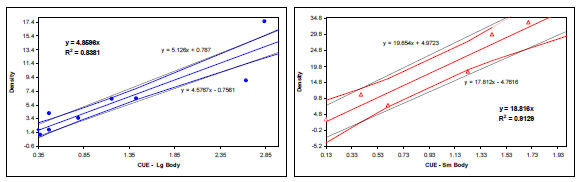
Relationship between density and CUE – SPIN(L2) only

Selectivity corrected area weighted index CUEs regressed against mark–recapture density estimates, separated by life history types (lake herring not present (small body) vs. lake herring present (large body)) are depicted in the figure above. A strong linear relationship exists between the two variables for both the large (R2 = 0.91) and small (R2 = 0.86) life history types; however, the relationships were observed to differ significantly (p = 0.010). The large bodied form was found to have approximately four times higher catchability than the small body form. This difference may be the result of a number of factors; 1. small bodied populations, which rarely exceed 450 mm, are vulnerable to fewer of the mesh panels than large body populations; 2. behaviour, likely associated with planktivorous foraging, may make small bodied fish less catchable. This could be the result of differences in encounter and retention rates with the gear, perhaps a consequence of a more circuitous movement pattern and/or slower swimming speed, or, a greater propensity for vertical orientation (i.e., greater proportion of population is off bottom); and 3. most likely, catchability of piscivorous lake trout is elevated by the presence of other fish in the net attracting them to it.
Hence, to be able to translate CUE into density, the specific life history type in the lake must be establish. Lakes that have herring (ciscoe), or other coregonids, are likely to be large bodied. In addition, populations were 50% female maturity (i.e., the smallest 25mm size class in which greater than 50% of females examined are mature, minimum of 10 samples) is attained at fork lengths greater than 500 mm are also likely to be large bodied systems. The Small Fish netting component and diet analysis are critical to include in a project if life history is unknown. In many systems herring are too small to be detected in the gear, but should be readily captured in the smaller Small Fish meshes and will be found in stomachs of the larger lake trout.
Equations to derive an estimated density from CUE are as follows:
Estimated Density Large Body = Adjusted CUE(L2) x 4.86
Estimated Density Small Body = Adjusted CUE(L2) x 18.82
There is error associated with both the estimation of the independent (density) and the dependent (CUE) variable in the calibration regression depicted above, to acknowledge this, a range of density for any particular lake should be reported along with the point estimate. However, the standard approach of using error associated with the overall lake CUE estimate (compounded by the heterogeneity of stratum densities) and the confidence limits of the calibration equation provide too expansive an interval to be of much practical use.

To provide an alternative approach, a study was undertaken by the Aquatic Science Unit to examine the level of measurement error associated with the CUE estimate. Standard SPIN surveys, as outlined in this report, were completed in an identical fashion over a period of four years in an experimental lake where exploitation pressure was negligible. Although the method and set locations remained constant, to incorporate any seasonal variability in catchability, the date when the survey was undertaken varied between years so that sampling span the full window of operation (three months). The lake was stocked annually with a fixed number of lake trout for a period of eight years prior to assessment and throughout the assessment period. Hence, it was assumed that the abundance of lake trout was relatively stable at the time of indexing and most of the variation in the observed CUE from year to year reflective of experimental error rather than actual changes in abundance. The 68% confidence interval (CI) was observed to be approximately eighteen percent of the mean (9% on either side), work is ongoing to evaluate this precision estimate. The 68% CI is suggested here, rather than the more typical 95%, as it provides a reasonable balance between the inherent high variability associated with measuring fish populations and the relatively low precision requirement when considering population estimates for recreational fisheries management.
| Year | Mean | Stdev | Month |
|---|---|---|---|
| 2003 | 1.61 | 1.86 | August |
| 2004 | 1.25 | 1.17 | July |
| 2005 | 1.74 | 1.36 | July |
| 2006 | 1.76 | 1.81 | September |
| Average | 1.59 | 1.55 |
68% min CL 1.45, 9%
68% max CL 1.73, 9%
Reversing the axes so that the relationship uses CUE (predictor) to estimate density (unknown), it is suggested that for reporting purposes the range of possible density in the lake be derived by assuming the above mentioned experimental error for the observed CUE and a 68% confidence interval associated with the density estimate. Confidence limits by nature are typically arced, to simplify density calculation a line was fitted to both the upper and lower CL to provide a linear approximation. The intersection of the minimum CUE and a best fit line for the lower confidence limit would provide a minimum density estimate. Intersection of the maximum CUE and best fit line of the upper confidence limit would provide a maximum density estimate.
Large (blue) and small (red) body calibration relationships with 68% CI and best fit lines
Following this approach, equations for calculating the range of possible density in a lake would be:

Overall abundance in numbers of fish for the lake can now be estimated by multiplying the minimum, mean and maximum point estimates by the area surveyed (not total lake area).
Work is underway to develop benchmarks for classifying the status of the lake using a combination of lake trout density, lake morphometry and species complex.
Appendix I - Bathymetric SPIN sampling map

Enlarge Bathymetric SPIN sampling map
Appendix II – Equipment list
- Anchors (2 per net)
- Boat/motor (and keys, chain and lock if needed)
- Catch and Set Sheets in clipboard
- Depth Sounder with Transducer (spare batteries if required)
- Echo Sounder (and paper)
- Floats (2 per net)
- Gas can with fuel line
- Gillnet gangs
- GPS with sites loaded (spare batteries if required)
- Life Jackets
- Measuring board Pencils and sharpie marker
- Ropes (of assorted lengths in tubs or pails)
- SPIN map with strata and sites (laminated)
- Bailing can
- Boat anchor
- Boat Hook Cell or
- Satellite phone
- Chain and lock for boats and motors
- Dip Net Field book
- First Aid Kit
- Knives
- Large Cooler with block of ice
- Navigational chart and Road Map
- Net picks
- Net tubs
- Paddles or oars
- Pails/plastic bags for sorting catch from
- Small Fish sets
- Rain/slime wear
- Rubber boots
- Scale Envelopes
- Sharpening stone
- Side Cutters
- Flat file
- Signalling device (whistle/horn)
- Thermistor Tool Kit
- Tweezers
- Weigh Scales
- Whirlpacks / labels
- YSI Oxygen Meter
Appendix III – Ontario species codes
Master List of Species Codes and Common Names of Ontario Fish (May 1998)
- Petromyzontidae - Lampreys
- American brook lamprey - Lampetra appendix
- northern brook lamprey - Ichthyomyzon fossor
- silver lamprey - Ichthyomyzon unicuspis
- sea lamprey - Petromyzon marinus
- Ichthyomyzon
- chestnut lamprey - Icthyomyzon castaneus
- Polyodontidae - Paddlefishes
- paddlefish - Polyodon spathula
- Acipenseridae - Sturgeons
- lake sturgeon - Acipenser fulvescens
- caviar
- Lepisosteidae – Gars
- longnose gar - Lepisosteus osseus
- spotted gar - Lepisosteus oculatus
- Lepisosteus sp.
- Amiidae - Bowfins
- bowfin - Amia calva
- Clupeidae – Herrings
- alewife - Alosa pseudoharengus
- American shad - Alosa sapidissima
- Gizzard shad - Dorosoma cepedianum
- Alosa sp.
Salmonidae - Trouts:
- Salmoninae - Salmon and Trout subfamily
- pink salmon - Oncorhynchus gorbuscha
- chum salmon - Oncorhynchus keta
- coho salmon - Oncorhynchus kisutch
- sockeye salmon - Oncorhynchus nerka
- chinook salmon - Oncorhynchus tshawytscha
- rainbow trout - Oncorhynchus mykiss
- Atlantic salmon - Salmo salar
- brown trout - Salmo trutta
- Arctic char - Salvelinus alpinus
- brook trout - Salvelinus fontinalis
- lake trout - Salvelinus namaycush
- splake - Salvelinus fontinalis x Salvelinus namaycush
- Aurora trout - Salvelinus fontinalis timagamiensis
- Oncorhynchus sp.
- Salmo sp.
- Salvelinus sp.
- Coregoninae - Whitefish subfamily
- lake whitefish - Coregonus clupeaformis
- longjaw cisco - Coregonus alpenae
- cisco (lake herring) - Coregonus artedi
- bloater - Coregonus hoyi
- deepwater cisco - Coregonus johannae
- kiyi - Coregonus kiyi
- blackfin cisco - Coregonus nigripinnis
- Nipigon cisco - Coregonus nipigon
- shortnose cisco - Coregonus reighardi
- shortjaw cisco - Coregonus zenithicus
- pygmy whitefish - Prosopium coulteri
- round whitefish - Prosopium cylindraceum
- chub - Coregonus (Cisco species other than C. artedi)
- Coregonus sp.
- Prosopium
- Thymallinae - Grayling subfamily
- Arctic grayling - Thymallus arcticus
- Osmeridae - Smelts
- rainbow smelt - Osmerus mordax
- Esocidae - Pikes
- northern pike - Esox lucius
- muskellunge - Esox masquinongy
- grass pickerel - Esox americanus vermiculatus
- Esox sp.
- chain pickerel - Esox niger
- Umbridae - Mudminnows
- central mudminnow - Umbra limi
- Hiodontidae - Mooneyes
- goldeye - Hiodon alosoides
- mooneye - Hiodon tergisus
- Catostomidae - Suckers
- quillback - Carpiodes cyprinus
- longnose sucker - Catostomus Catostomus
- white sucker - Catostomus commersoni
- lake chubsucker - Erimyzon sucetta
- northern hog sucker - Hypentelium nigricans
- bigmouth buffalo - Ictiobus cyprinellus
- spotted sucker - Minytrema melanops
- silver redhorse - Moxostoma anisurum
- black redhorse - Moxostoma duquesnei
- golden redhorse - Moxostoma erythrurum
- shorthead redhorse - Moxostoma macrolepidotum
- greater redhorse - Moxostoma valenciennesi
- river redhorse - Moxostoma carinatum
- black buffalo - Ictiobus niger
- Catostomus sp.
- Moxostoma sp.
- Ictiobus sp.
- Cyprinidae - Carps and Minnows
- goldfish - Carassius auratus
- northern redbelly dace - Phoxinus eos
- finescale dace - Phoxinus neogaeus
- redside dace - Clinostomus elongatus
- lake chub - Couesius plumbeus
- common carp - Cyprinus carpio
- gravel chub - Erimystax x punctatus
- cutlips minnow - Exoglossum maxillingua
- brassy minnow - Hybognathus hankinsoni
- eastern silvery minnow - Hybognathus regius
- silver chub - Macrhybopsis storeriana
- hornyhead chub - Nocomis biguttatus
- river chub - Nocomis micropogon
- golden shiner - Notemigonus crysoleucas
- pugnose shiner - Notropis anogenus
- emerald shiner - Notropis atherinoides
- bridle shiner - Notropis bifrenatus
- common shiner - Luxilus cornutus
- blackchin shiner - Notropis heterodon
- blacknose shiner - Notropis heterolepis
- spottail shiner - Notropis hudsonius
- rosyface shiner - Notropis rubellus
- spotfin shiner - Cyprinella spiloptera
- sand shiner - Notropis stramineus
- redfin shiner - Lythrurus umbratilis
- mimic shiner - Notropis volucellus
- pugnose minnow - Opsopoeodus emiliae
- bluntnose minnow - Pimephales notatus
- fathead minnow - Pimephales promelas
- blacknose dace - Rhinichthys atratulus
- longnose dace - Rhinichthys cataractae
- creek chub - Semotilus atromaculatus
- fallfish - Semotilus corporalis
- pearl dace - Margariscus margarita
- silver shiner - Notropis photogenis
- central stoneroller - Campostoma anomalum
- striped shiner - Luxilus chrysocephalus
- ghost shiner - Notropis buchanani
- grass carp - Ctenopharyngodon idella
- rudd - Scardinius erythrophthalmus
- Phoxinus sp.
- Hybognathus sp.
- Nocomis sp.
- Notropis sp.
- Pimephales sp.
- Rhinichthys sp.
- Semotilus sp.
- Hybopsis sp.
- Luxilus sp.
- Ictaluridae - Bullhead Catfishes
- black bullhead - Ameiurus melas
- yellow bullhead - Ameiurus natalis
- brown bullhead - Ameiurus nebulosus
- channel catfish - Ictalurus punctatus
- stonecat - Noturus flavus
- tadpole madtom - Noturus gyrinus
- brindled madtom - Noturus miurus
- margined madtom - Noturus insignis
- flathead catfish - Pylodictis olivaris
- Ictalurus sp.
- Noturus sp.
- Ameiurus sp.
- northern madtom - Noturus stigmosus
- Anguillidae - Freshwater Eels
- American eel - Anguilla rostrata
- Cyprinodontidae - Killifishes
- banded killifish - Fundulus diaphanus
- blackstripe topminnow - Fundulus notatus
- Gadidae - Cods
- burbot - Lota lota
- Gasterosteidae - Sticklebacks
- brook stickleback - Culaea inconstans
- threespine stickleback - Gasterosteus aculeatus
- ninespine stickleback - Pungitius pungitius
- fourspine stickleback - Apeltes quadracus
- Percopsidae - Trout-perches
- trout-perch - Percopsis omiscomaycus
- Percichthyidae - Temperate Basses
- white perch - Morone americana
- white bass - Morone chrysops
- Morone sp.
- Centrarchidae - Sunfishes
- rock bass - Ambloplites rupestris
- green sunfish - Lepomis cyanellus
- pumpkinseed - Lepomis gibbosus
- blue gill - Lepomis macrochirus
- longear sunfish - Lepomis megalotis
- smallmouth bass - Micropterus dolomieu
- largemouth bass - Micropterus salmoides
- white crappie - Pomoxis annularis
- black crappie - Pomoxis nigromaculatus
- Lepomis sp.
- Micropterus sp.
- Pomoxis sp.
- warmouth - Lepomis gulosus
- orangespotted sunfish - Lepomis humilis
- Percidae - Perches
- yellow perch - Perca flavescens
- sauger - Stizostedion canadense
- blue pike (blue pickerel) - Stizostedion vitreum glaucum
- walleye (yellow pickerel) - Stizostedion vitreum
- eastern sand darter - Ammocrypta pellucida
- greenside darter - Etheostoma blennioides
- rainbow darter - Etheostoma caeruleum
- Iowa darter - Etheostoma exile
- fantail darter - Etheostoma flabellare
- least darter - Etheostoma microperca
- johnny darter - Etheostoma nigrum
- logperch - Percina caprodes
- channel darter - Percina copelandi
- blackside darter - Percina maculata
- river darter - Percina shumardi
- tessellated darter - Etheostoma olmstedi
- Stizostedion sp.
- Etheostoma sp.
- Percina sp.
- ruffe - Gymnocephalus cernuus
- Atherinidae - Silversides
- brook silverside - Labidesthes sicculus
- Gobiidae – Gobies
- round goby - Neogobius melanostomus
- tubenose goby - Proterorhinus marmoratus
- Sciaenidae - Drums
- freshwater drum - Aplodinotus grunniens
- Cottidae - Sculpins
- mottled sculpin - Cottus bairdi
- slimy sculpin - Cottus cognatus
- spoonhead sculpin - Cottus ricei
- deepwater sculpin - Myoxocephalus thompsoni
- Cottus sp.
- Myoxocephalus sp.
- fourhorn sculpin - Myoxocephalus quadricornis
- Cyclopteridae - Lumpfishes
- lumpfish - Cyclopterus lumpus
- Pleuronectidae - Righteye Flounders
- European Flounder - Platichthys flesus
- Salmonidae - Hybrids
- Salmoninae - Hybrids
- Coregoninae - Hybrids
- Esocidae - Hybrids
- Esox lucius x Esox americanus vermiculatus
- Esox lucius x Esox masquinongy
- Catostomidae - Hybrids
- Ictiobus hybrids
- Cyprinidae - Hybrids
- Carassius auratus x Cyprinus carpio
- Phoxinus hybrids Phoxinus eos x Phoxinus neogaeus
- Phoxinus eos x Margariscus margarita
- Phoxinus neogaeus x Margariscus margarita
- Notropis hybrids
- Luxilus cornutus x Notropis rubellus
- Luxilus cornutus x Semotilus atromaculatus
- Pimephales promelas x Pimephales notatus
- Ictaluridae - Hybrids
- Ameiurus melas x Ameiurus nebulosus
- Centrarchidae - Hybrids
- Lepomis hybrids
- Lepomis gibbosus x Lepomis macrochirus
- Lepomis cyanellus x Lepomis gibbosus
- Lepomis cyanellus x Lepomis megalotis
- Lepomis cyanellus x Lepomis macrochirus
- Pomoxis annularis x Pomoxis nigromaculatus
- Percidae – Hybrids
- Stizostedion canadense x Stizostedion vitreum
- Cottidae - Hybrids
- Cottus bairdi x Cottus cognatus
Appendix IV - Example of completed set and catch forms
Example of completed set and catch forms
Appendix V – Table of Ontario Lakes with SPIN surveys (up to 2006)
| Lake | Year | Zone | Northing | Easting | L/H type | Stocked | Lake Area | Strata Area (optimal habitat ha) 10_20 | Strata Area (optimal habitat ha) 20_30 | Strata Area (optimal habitat ha) 30_40 | Strata Area (optimal habitat ha) 40_60 | Strata Area (optimal habitat ha) 60_80 | Strata Area (optimal habitat ha) 80+ | CUE >300 area wt sel corrected Est 1 | CUE >300 area wt sel corrected Est 2 | CUE >300 area wt sel corrected Est 3 | CUE >300 area wt sel corrected Est 4 | CUE >300 area wt sel corrected Est 5 | Avg. CUE |
|---|---|---|---|---|---|---|---|---|---|---|---|---|---|---|---|---|---|---|---|
| Ashby | 2006 | 18 | 315009 | 4995938 | SB | no | 260 | 111 | 36 | 8 | 0.51 | 0.51 | |||||||
| Bella | 2006 | 17 | 654803 | 5034569 | LB | yes | 328 | 114 | 52 | 21 | 0.82 | 0.82 | |||||||
| Bernard | 2006 | 17 | 626530 | 5065169 | LB | no | 2058 | 401 | 302 | 133 | 194 | 1.52 | 1.52 | ||||||
| Big Salmon | 2006 | 18 | 382059 | 4933586 | LB | no | 148 | 37 | 28 | 28 | 5 | 1.54 | 1.54 | ||||||
| Big Wind | 2005 | 17 | 652934 | 4991004 | LB | yes | 107 | 24 | 12 | 7 | 0.06 | 0.06 | |||||||
| Boshkung | 2006 | 17 | 678931 | 4990848 | LB | no | 716 | 117 | 124 | 117 | 142 | 5 | 2.40 | 2.40 | |||||
| Camp | 2004 | 17 | 663745 | 5033965 | SB | no | 189 | 45 | 21 | 22 | 0.44 | 0.44 | |||||||
| Canoe | 2005 | 18 | 377690 | 4939819 | SB | no | 291 | 65 | 59 | 53 | 46 | 1.75 | 1.75 | ||||||
| Dickey | 2003–04 | 18 | 282976 | 4963418 | SB | no | 208 | 50 | 43 | 23 | 0.33 | 0.66 | 0.50 | ||||||
| Dotty | 2005 | 17 | 657627 | 5035535 | LB | yes | 153 | 29 | 9 | 0.66 | 0.66 | ||||||||
| Drag | 2002 06 | 17 | 702697 | 4992644 | LB | no | 1003 | 220 | 250 | 100 | 0.34 | 0.64 | 0.49 | ||||||
| Essen | 2006 | 17 | 714068 | 4990707 | SB | yes | 245 | 66 | 47 | 8 | 0.53 | 0.53 | |||||||
| Fairy | 2003–05 | 17 | 644388 | 5021787 | LB | yes | 712 | 177 | 93 | 76 | 70 | 67 | 1.50 | 1.87 | 1.20 | 1.45 | 1.51 | ||
| Faraday | 2005 | 18 | 269376 | 4994347 | LB | no | 114 | 48 | 4 | 0.21 | 0.21 | ||||||||
| Farquhar | 2006 | 17 | 720982 | 4997091 | SB | no | 336 | 77 | 83 | 61 | 0.29 | 0.29 | |||||||
| Fletcher | 2005 | 17 | 672323 | 5024267 | LB | yes | 256 | 77 | 5 | 0.47 | 0.47 | ||||||||
| Gilles | 2005–06 | 17 | 474385 | 5005255 | LB | yes | 214 | 22 | 37 | 4 | 2.10 | 1.01 | 1.56 | ||||||
| Grace | 2006 | 17 | 716708 | 4995361 | SB | yes | 226 | 80 | 40 | 18 | 0.21 | 0.21 | |||||||
| Grass | 2004 | 17 | 639874 | 5060986 | LB | no | 135 | 35 | 27 | 5 | 0.81 | 0.81 | |||||||
| Greenwater | 2005 | 15 | 687195 | 5385721 | LB | no | 3060 | 984 | 739 | 454 | 198 | 0.76 | 0.76 | ||||||
| Grouse | 2003 | 15 | 681726 | 5878455 | SB | no | 87 | 24 | 16 | 15 | 0.83 | 0.83 | |||||||
| Halls | 2005 | 17 | 678492 | 4996841 | SB | no | 543 | 107 | 91 | 95 | 114 | 18 | 0.34 | 0.34 | |||||
| Island | 2005 | 17 | 636893 | 5060024 | LB | yes | 127 | 49 | 12 | 0.04 | 0.04 | ||||||||
| Joseph | 2003–06 | 17 | 597617 | 5011850 | LB | no | 5156 | 1337 | 810 | 534 | 3.81 | 3.09 | 3.31 | 2.30 | 3.13 | ||||
| Kawagama | 2004–06 | 17 | 674693 | 5016101 | SB | no | 2819 | 535 | 512 | 207 | 0.89 | 0.57 | 0.92 | 0.79 | |||||
| Kimball | 2006 | 17 | 681331 | 5023064 | SB | no | 213 | 46 | 49 | 25 | 33 | 0.32 | 0.32 | ||||||
| Koshlong | 2003 05 | 17 | 698791 | 4982604 | LB | yes | 401 | 94 | 30 | 24 | 0.78 | 0.85 | 0.82 | ||||||
| Lake of Bays | 2004 | 17 | 657061 | 5012277 | LB | no | 6904 | 1309 | 1080 | 832 | 1116 | 0.78 | 0.78 | ||||||
| L of the Woods (Whitefish Bay) | 2005 | 15 | 418140 | 5472322 | LB | no | 22000 | 2000 | 3532 | 2208 | 0.99 | 0.99 | |||||||
| Lake Simcoe | 2005 | 17 | 630247 | 4919755 | LB | yes | 72500 | 19587 | 10882 | 6529 | 1.07 | 1.07 | |||||||
| Lake St Peter | 2006 | 17 | 732979 | 5021317 | SB | yes | 231 | 61 | 23 | 0.16 | 0.16 | ||||||||
| L’Amable | 2006 | 18 | 277419 | 4988479 | SB | yes | 178 | 40 | 23 | 15 | 0.24 | 0.24 | |||||||
| Lobster | 2006 | 17 | 717753 | 5046960 | LB | yes | 133 | 49 | 8 | 1.08 | 1.08 | ||||||||
| Loughborough | 2006 | 18 | 380567 | 4916747 | LB | yes | 738 | 190 | 140 | 70 | 0.81 | 0.81 | |||||||
| Louisa | 2003 | 17 | 697479 | 5038469 | SB | no | 718 | 125 | 91 | 39 | 0.66 | 0.66 | |||||||
| Mary | 2003–06 | 17 | 635467 | 5010598 | LB | yes | 1065 | 195 | 205 | 106 | 280 | 1.61 | 1.25 | 1.74 | 1.76 | 1.59 | |||
| Miskwabi | 2006 | 17 | 711585 | 4993161 | SB | yes | 264 | 71 | 55 | 47 | 0.36 | 0.36 | |||||||
| Muskoka | 2003 05 | 17 | 618483 | 4991664 | LB | yes | 12206 | 3119 | 1499 | 1312 | 0.97 | 1.01 | 0.99 | ||||||
| Opeongo | 2003 | 17 | 704578 | 5062061 | LB | no | 5154 | 1718 | 740 | 646 | 1.97 | 1.97 | |||||||
| Papineau | 2005 | 18 | 279212 | 5023845 | SB | no | 831 | 246 | 124 | 36 | 128 | 4 | 0.78 | 0.78 | |||||
| Peninsula | 2003–05 | 17 | 646983 | 5022655 | LB | yes | 865 | 184 | 102 | 56 | 1.30 | 1.83 | 1.30 | 1.48 | |||||
| Portage | 2005 | 17 | 594351 | 5007173 | LB | yes | 98 | 39 | 13 | 0.52 | 0.52 | ||||||||
| Rebecca | 2005 | 17 | 653140 | 5032783 | LB | yes | 211 | 49 | 12 | 0.91 | 0.91 | ||||||||
| Rosseau | 2002–2006 | 17 | 611898 | 4999461 | LB | no | 6374 | 1357 | 1210 | 679 | 2.62 | 3.63 | 2.94 | 2.11 | 2.16 | 2.69 | |||
| Sand | 2005 | 17 | 643643 | 5054532 | LB | yes | 568 | 137 | 138 | 75 | 1.01 | 1.01 | |||||||
| Skeleton | 2004 | 17 | 620069 | 5010117 | LB | no | 2156 | 338 | 170 | 206 | 1.20 | 1.20 | |||||||
| Smoke | 2003 | 17 | 681044 | 5043357 | LB | no | 607 | 178 | 81 | 79 | 0.94 | 0.94 | |||||||
| Soyers | 2006 | 17 | 688330 | 4987799 | LB | no | 331 | 58 | 34 | 23 | 0.36 | 0.36 | |||||||
| Spring | 2006 | 17 | 603220 | 5074198 | LB | no | 244 | 49 | 33 | 16 | 28 | 0.91 | 0.91 | ||||||
| Squeers | 2003 05 | 15 | 680317 | 5376668 | SB | no | 384 | 180 | 50 | 1.36 | 1.86 | 1.61 | |||||||
| Temagami | 2006 | 17 | 573726 | 5204366 | LB | no | 22654 | 6426 | 2935 | 1873 | 2737 | 424 | 1.56 | 1.56 | |||||
| Twelve Mile | 2005 06 | 17 | 681198 | 4989806 | LB | no | 337 | 132 | 58 | 0.98 | 0.89 | 0.94 | |||||||
| Upper Medicine Stone | 2004 | 15 | 422685 | 5642266 | LB | no | 1073 | 290 | 215 | 143 | 0.60 | 0.60 | |||||||
| Vernon | 2004–05 | 17 | 634599 | 5021144 | LB | yes | 1505 | 407 | 232 | 209 | 0.61 | 1.24 | 0.93 | ||||||
| Wahnapitae | 2006 | 17 | 522580 | 5173609 | LB | no | 19357 | 2046 | 1308 | 1340 | 1987 | 1844 | 1570 | 0.62 | 0.62 | ||||
| Wawashkesh | 2004 | 17 | 575918 | 5060044 | LB | no | 1720 | 200 | 120 | 90 | 0.09 | 0.09 | |||||||
| Weslemkoon | 2006 | 18 | 309251 | 4991580 | SB | no | 1955 | 555 | 160 | 31 | 0.75 | 0.75 |
Appendix VI – Table of lakes outside Ontario with SPIN surveys (up to 2006)
| Lake | Year | Zone | Northing | Easting | L/H type | Stocked | Lake Area | Strata Area (optimal habitat ha) 10_20 | Strata Area (optimal habitat ha) 20_30 | Strata Area (optimal habitat ha) 30_40 | Strata Area (optimal habitat ha) 40_60 | Strata Area (optimal habitat ha) 60_80 | Strata Area (optimal habitat ha) 80+ | CUE >300 area wt sel corrected Est 1 | CUE >300 area wt sel corrected Est 2 | CUE >300 area wt sel corrected Est 3 | CUE >300 area wt sel corrected Est 4 | CUE >300 area wt sel corrected Est 5 | Avg. CUE |
|---|---|---|---|---|---|---|---|---|---|---|---|---|---|---|---|---|---|---|---|
| Caugnawana (PQ) | 2005 | 17 | 705244 | 5158302 | SB | no | 790 | 196 | 39 | 1.97 | 1.97 | ||||||||
| Maganasipi (PQ) | 2006 | 17 | 700226 | 5156842 | SB | no | 934 | 340 | 94 | 32 | 33 | 1.87 | 1.87 | ||||||
| Binta (BC) | 2006 | 10 | 333676 | 5974197 | LB | no | 739 | 261 | 201 | 85 | 0.85 | 0.85 | |||||||
| Crean (SK) | 2005 | 13 | 417772 | 5991697 | LB | no | 12075 | 551 | 1002 | 0.09 | 0.09 | ||||||||
| Minnewanka (AB) | 2005 06 | 11 | 618645 | 5677832 | LB | no | 2100 | 229 | 385 | 238 | 375 | 196 | 310 | 3.76 | 2.65 | 3.21 | |||
| Uncha (BC) | 2006 | 10 | 328947 | 5976927 | LB | no | 1383 | 407 | 395 | 131 | 1.27 | 1.27 | |||||||
| Wassegam (SK) | 2006 | 13 | 418060 | 6015729 | LB | no | 1027 | 285 | 374 | 98 | 3.13 | 3.13 |