Technical Bulletin: modelling open flares under O.Reg. 419/05
This technical bulletin will assist modellers by providing the appropriate approach for modelling open flares using approved air dispersion models (e.g. AERMOD or SCREEN3 ) under O.Reg. 419/05.
Executive Summary
This Technical Bulletin has been developed to outline the approach for modelling open flares and clarifies some technical issues related to how these sources are to be characterized in advanced
A tiered modelling approach is presented in this Technical Bulletin, beginning with a simplified assessment and progressing to more refined modelling assessments if the initial assessment results in Point of Impingement (POI) concentrations which may exceed Ministry of the Environment and Climate Change (the Ministry) O. Reg. 419/05 air standard(s) or guideline(s). As with other Ministry standards or guidelines, if refined modelling indicates an exceedence of an air standard or guideline, notification under section 28 of O. Reg. 419/05 is required.
This Technical Bulletin also outlines the process for calculating flare pseudo-parameters which are used to model open flares as point sources using AERMOD or another approved, advanced air dispersion model under O. Reg. 419/05. Appropriate characterization of pseudo-parameters is required to reasonably represent emission source characteristics associated with open flares such that plume behaviour (plume rise and plume spread) and resulting POI concentrations are adequately represented when these parameters are input into advanced air dispersion models. The primary goal of this Technical Bulletin is to outline a consistent calculation approach for these pseudo-parameters.
The approach presented in this Technical Bulletin is targeted to facilities subject to Schedule 3 standards, as per section 20 of O. Reg. 419/05. It can also be used by facilities that are subject to the ½-hour standards in Schedule 2, as per section 19 of O. Reg. 419/05. Facilities operating under section 19 of O. Reg. 419/05 (i.e. subject to ½-hour standards in Schedule 2) may also use this approach with SCREEN3 or an advanced air dispersion model such as AERMOD. These models calculate the maximum 1-hour POI concentration of each contaminant, which must then be converted to a ½-hour maximum POI concentration using the equation presented in section 17 of O. Reg. 419/05. Alternately, facilities can request a speed up under subsection 20(4) to have a Schedule 3 standard apply to the contaminant(s) in question, in advance of their February 1st, 2020 phase-in date.
In addition to this Technical Bulletin, the Ministry guideline document entitled “Air Dispersion Modelling Guideline for Ontario (ADMGO)”, (as amended), provides guidance on the appropriate meteorological data, approved dispersion models, and other modelling parameters and approaches that are to be considered in the implementation of Ministry O. Reg. 419/05 standards and guidelines. The Ministry guideline document entitled “Procedure for Preparing and Emission Summary and Dispersion Modelling Report” (as amended) provides guidance on determination of appropriate emission rates.
It should also be noted that this Technical Bulletin does not address the modelling of closed flares. Closed flares behave similarly to normal point sources, and therefore can be modelled as such. This Technical Bulletin only provides guidance for modelling assessments of open flares.
Challenges With Modelling Open Flares
The main challenge related to modelling open flares is the fact that most models do not specifically have an open flare source type. Instead, the flare emissions are modelled as point sources. The exhaust characteristics of open flares however, are quite different from traditional “stack type” point source exhaust streams. Open flares produce extremely hot (and therefore buoyant), turbulent exhaust streams. Also, open flares typically have a jet-like flame, and exhaust/combustion contaminants are emitted from a plume that starts at the top of the flame, or the flame tip. These exhaust characteristics therefore necessitate the calculation and use of exhaust effective “pseudo-parameters” to appropriately characterize the flare in order to ensure that the resulting plume rise and plume spread are reasonably representative. Some models, such as SCREEN3, calculate pseudo-parameters internally, but may use different approaches than those detailed in Chapter 2 of this Technical Bulletin. Other models, such as AERMOD, do not automatically calculate these pseudo-parameters, and therefore they must be calculated externally (i.e. outside of the model). As a result, the Ministry has developed this Technical Bulletin to outline the recommended approach for modelling open flares.
1.1 Use of SCREEN3
The SCREEN3 model has a built-in flare source type and automatically calculates and utilizes relatively conservative values for some of the pseudo-parameters. This provides an easy-to-use method of obtaining contaminant concentration estimates and can be used to provide an initial screening assessment of POI concentrations from an open flare. If a proponent uses SCREEN3 to model open flares, the built-in flare source type in SCREEN3 must be used as is. It is not appropriate for proponents to use a point source type with externally calculated pseudo-parameters for SCREEN3.
1.2 Use of Advanced Air Dispersion Models
Advanced air dispersion models such as AERMOD and CALPUFF use hourly meteorological observations to calculate contaminant dispersion and resulting POI concentrations. These models either do not have built-in flare source types, and therefore do not calculate the necessary flare pseudo-parameters, or use a different approach to calculate these parameters. When these models are used, the approach and equations outlined in chapter 2 of this Technical Bulletin are to be used to characterize the source parameters.
Note that commercial user interfaces for these models may also have “flare” sources, which are treated similarly to the approach used by SCREEN3. As such, these programs will calculate the pseudo-parameters automatically. However, as of the date of this Technical Bulletin, these interfaces do not follow the specific calculation methodology provided in this Technical Bulletin and as such should not be used without first obtaining written agreement from the Ministry’s Environmental Monitoring and Reporting Branch.
Procedures For Modelling Open Flares When Using Advanced Air Dispersion Models
The following chapters provide further details on the technical challenges associated with modelling open flares using advanced air dispersion models, and the approach to be used in such assessments under O. Reg. 419/05.
2.1 Background on Open Flares and Effective Parameters
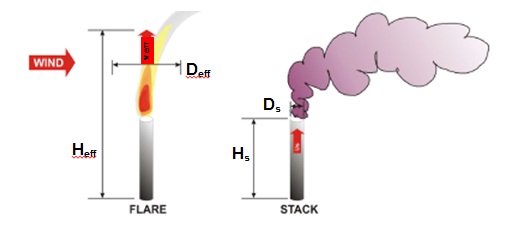
Open flares at industrial facilities are typically used for the destruction or disposal of combustible vent gases. Because these streams are burned in an open, jet-type flame, flare exhaust tends to be very hot, and is subject to both buoyant, and to a lesser extent, momentum rise. Also, as the flame burns, air is entrained to supply the oxygen needed for combustion. Typically, excess air is entrained, which increases the initial volume of the exhaust gas, and lowers the temperature. Heat is also lost by thermal radiation, which further lowers the temperature of the plume. This typically results in exhaust gas temperatures ranging from 650 to 1000°C, at the end of the flame. Briggs plume rise equations can be used to determine the final rise of plumes within this temperature range (Beychok, 1979). As a result, the combusted gas plume rise from a flare stack is generally defined as starting at the flame tip. Because of this assumption, the flare stack height must be increased to account for the additional height of the flame (or “flame length”) when modelling an open flare as a point source with advanced air dispersion models. In addition, all other required source parameters (temperature, diameter, exit velocity) must be determined or calculated at the flame tip, as opposed to the flare nozzle tip. These parameters include the following:
- Modified or “effective” stack height (Heff)
- Effective Exit Velocity (Veff)
- Effective Stack Diameter (Deff)
These are known as pseudo-parameters, and they do not necessarily have any physical relevance (i.e. Deff is not a real diameter of the stack or flame/plume width). They are calculated in a manner to simulate the behaviour of the exhaust plume as if it were a point source, emitted at the tip of the flame, from a stack with a diameter that is based on a calculated size/spread of the plume at the flame tip, and with an exit velocity that considers the expected expansion and air entrainment, but conserves buoyancy and momentum flux. The intent is to determine a combination of pseudo-parameters that result in a model calculated plume rise that is reasonable. As such, appropriate calculation of these pseudo-parameters is particularly important. Previous approaches may have resulted in overestimates of the final plume rise, which would generally result in underestimates of maximum point of impingement concentrations.
Figure 1 illustrates the differences between flare stacks and point source stacks.
Figure 1 – Differences between Flare and Point Source
These pseudo-parameters are calculated as outlined in the following chapters, and input directly into an advanced air dispersion model such as AERMOD as point source exhaust characteristics. In this manner, the plume rise and dispersion calculations are performed as if the flare behaves as a typical point source.
2.2 Calculation of Flare Effective Pseudo-Parameters
2.2.1 Effective Stack Height (Heff)
The effective stack height is the total height of the flare, including the height of the flame. It is calculated using the physical height of the flare in addition to the flame length. The flame length is dependent upon the net heat release rate and the flame tilt due to the wind. The stronger the wind, the greater the flame tilt, and the shorter the resulting vertical flame length. In order to simplify the calculations, it has been assumed that the wind speed is sufficient to tilt the flame at a 45° angle, which is a reasonably conservative assumption. The net heat release rate considers the total amount of heat available through combustion, minus the amount lost through radiation (ƒ). Some flares burn quite cleanly, and produce no visible plume, while others are very smoky or sooty. Flares with smoky, dark plumes lose more heat through radiation than cleaner, more transparent plumes (Leahey and Davies, 1984).
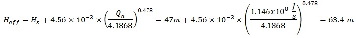
The equation used to estimate the effective stack height is as follows:
Equation 1:
Heff = Hs + 4.56 × 10⁻³ × (Qn ÷ 4.1868)0.478
Qn = QT × (1 − ƒ)
Where:
- Hs
- physical stack height above ground (m)
- Heff
- effective stack height, includes the physical stack height plus
- includes the flame length, and assumes 45° flame tilt due to wind
- QT
- total heat available from combustion, in Joules/second (J/s)
- Sensible and radiative heat available estimated based on the properties of the flared gas stream including the pilot fuel and combustible lift gas
- ƒ
- % heat lost by radiation
- A function of the molecular weight (MW) of the flared gas stream
- Flares with smoky, dark plumes lose more heat via radiation (i.e. higher value for ƒ) than clean burning flares with no visible plumes
- Qn
- net heat released (J/s)
While it is recognized that the burning and operational conditions of the flare have an effect on the smokiness and therefore the radiative heat loss, this has not been considered for the purposes of these calculations.
A number of studies have attempted to quantify the relationship between flare burning conditions, radiative heat losses and plume rise. The most commonly cited study is that by Leahey and Davies, 1984. Their study focussed on visual observations of plume rise through rapid photography, which were then correlated to the burning conditions, to derive values for radiative heat loss. However, it should be noted that since the study used visual observations of the plume and plume height, a relatively heavy oil (approximately equivalent in molecular weight to Bunker B fuel) was added to the flame to intentionally make it smoke, such that the extent of plume rise was clear. This significantly increased the effective MW of the stream (i.e. flared gas plus oil). The results of this study indicate that the flare lost 55% of the total available heat through radiative losses. This value of 55% radiative heat loss is used today by various regulatory agencies (e.g. SCREEN3 model), and is typically regarded as a conservative screening value. Other regulatory agencies, such as Alberta Environment recommend use of an ƒ value of 25% radiative heat loss, which is more consistent with ƒ values as presented in the literature for specific flared gas streams.
Other researchers, such as Tan, 1967, developed an empirical relationship between the MW of the flared gas stream and the fraction of radiative heat losses. The values produced by Tan are typical of those seen in the literature for the composition of various flare gas streams. Tan’s empirical relationship has been incorporated into the calculation of flare pseudo-parameters in the state of Texas (TCEQ, 2004). Other jurisdictions, such as the San Joachim Valley, CA, provide specific values of ƒ for specific fuels or flared gas streams.
The Ministry has adopted a hybrid approach, based on a combination of the Tan relationship and the range of ƒ values published in the peer-reviewed literature. This is presented in Table 1 as specified ranges of molecular weights of the gas stream to be flared corresponding to a given ƒ value. This simple approach affords the flexibility to use a scientifically-based stream-specific radiative heat loss value, while still maintaining a reasonable amount of conservatism.
| Molecular Weight (gram/mole) | Radiative heat loss values (ƒ) |
|---|---|
| ≤ 20 | 25% |
| 21 - 35 | 30% |
| 36 - 50 | 35% |
| 51 - 65 | 40% |
| 66 - 80 | 45% |
| 81 - 95 | 50% |
| > 95 | 55% |
Proponents should calculate the MW of their flared gas stream, based on the documented and/or measured composition considering all potential chemical constituents (e.g. flare gas, non-inert lift or sweep gas, etc.) and then select the corresponding ƒ value. The composition of the stream to be flared, including the ratio of non-inert lift and/or sweep gas to flare gas, must be consistent with the scenario(s) being assessed (i.e. if different processes or vessels depressurize and result in different flaring events, these may need to be assessed individually). In addition, proponents should calculate the Lower Explosive Limit (LEL)
Note that while monitoring for stream composition and flow rate is the most accurate method of determining MW, it is not required under this Technical Bulletin. Engineering estimates based on conservative design simulations can also provide a reasonable estimate of MW under different scenarios. Fulsome documentation/rationale for each scenario and estimate, as well as sample calculations must be provided to the ministry.
2.2.2 Effective Exit Velocity (Veff)
The effective exit velocity is calculated as a representative value at the flame tip. When the gas burns, the size of the flame and exhaust gases (in terms of the stack diameter or area) is much larger than the original inner diameter of the open flare or flare nozzle tip. This is due to the combustion process and air entrainment in the plume at the flame tip.
The key parameter that has historically been used to calculate pseudo-parameters for open flares is buoyancy flux (Fb). Fb is a measure of the “lift rate” that the exhaust gas has due to the amount of heat released through combustion. Some jurisdictions however, have recommended the use of the actual gas exit velocity at the flare nozzle tip rather than an effective exit velocity.
Alberta Environment, for example, previously used this approach (i.e. actual nozzle exit velocity) in its former methodology for calculating flare pseudo-parameters
In actuality, these combinations of conditions are not likely to occur, since the entrained air would serve to cool the exhaust stream somewhat and reduce Fb. The main problem is that there is no simple way to determine (or approximate) how much air is entrained. Instead, some jurisdictions use a slightly more conservative approach where the exit velocity is set to 20 m/s as is done in the SCREEN3 model, and by jurisdictions that follow the US EPA screening approach for flares. Use of this Veff value of 20 m/s however appears to be based on a design wind speed selected to prevent stack tip downwash (TCEQ, 2004), and may not be appropriate for use in Ontario. Also, the differing approaches previously used for selecting Veff have resulted in inconsistent Veff values being used in dispersion modelling assessments of flaring in Ontario. This Technical Bulletin provides a consistent methodology to be used when assessing open flares in Ontario.
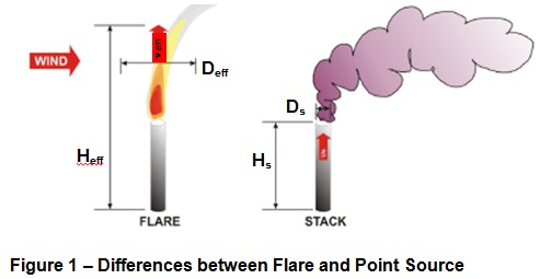
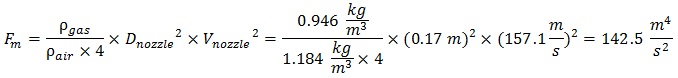
In addition, the effects of momentum flux (Fm) on the pseudo-parameters have been ignored in previous approaches. Calculation of pseudo-parameters without consideration of Fm has in part contributed to an overestimation in plume rise. The Fm is a measure of “lift rate” that the gas has due to the amount of physical momentum of the stream (i.e. how fast the stream is released). Alberta Environment recently revised its approach for the calculation of flare pseudo-parameters to include a calculation methodology to approximate Veff at the flame tip. This approach considers the conservation of both buoyancy flux and momentum flux in the calculations. Both of these parameters can be determined for gas streams to be flared. Proponents calculate the momentum flux of the exhaust stream at the nozzle tip prior to combustion, as follows:
Equation 2: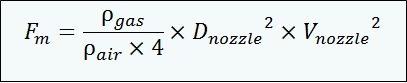
Where:
- Fm
- momentum flux (m4/s2)
- ρgas, ρair
- density of gas to be flared
footnote 4 , and ambient airfootnote 5 (kg/m3) - Dnozzle
- flare nozzle diameter (m)
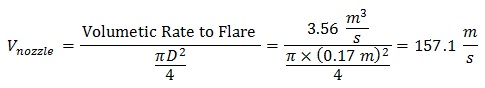
- Vnozzle
- actual gas exit velocity (including lift gas) at flare nozzle before combustion
footnote 6 (m/s)
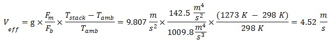
Note again that the momentum flux (Fm) is calculated based on the parameter values at the flare nozzle tip. The exhaust stream at this location behaves similar to a traditional stack. This momentum flux is assumed to be conserved, and therefore is also applicable at the flame tip. Thus, it can be used to calculate the effective velocity, as per the following equation:
Equation 3:
Where:
- Veff
- effective velocity at the flame tip (m/s) [minimum value = 1.5 m/s]
- g
- acceleration due to gravity (9.81 m/s2)
- Fb
- buoyancy flux (m4/s3)
- Tstack
- combusted gas temperature (MOECC assumes 1273 K)
- Tamb
- ambient temperature (K)
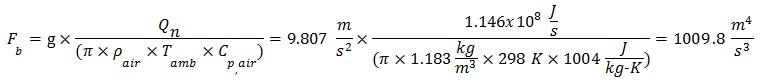
The buoyancy flux (Fb, actual) of the combusted gas is calculated as follows:
Equation 4: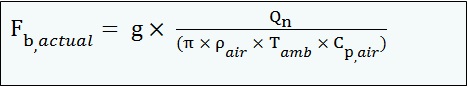
Where:
- Qn
- net heat release rate (J/s) (see Eqn (1))
- ρair
- density of air at ambient temperature and pressure (kg/m3)
- Cp,air
- specific heat of dry air constant at Tamb (J/kg-K)
Note that the minimum value of Veff is 1.5 m/s to prevent stack tip downwash during calms and low wind speed events.
It should be noted that flares are typically sized to accommodate flows during non-routine events that are much larger than those experienced during routine flare operations (e.g. “turn down”, “pilot” modes). As a result, during routine flare operations, the nozzle velocity and associated momentum flux are much lower than that during non-routine events. Because of this, the estimates of Veff for flares designed for larger, non-routine events are expected to be much lower during routine flare operations. This would lead to modelled plume rises that are appropriately reduced in comparison to non-routine operations.
2.2.3 Effective Stack Diameter (Deff)
Similar to the effective exit velocity, the effective stack diameter is calculated at the flame tip. One of the key parameters used to calculate the effective stack diameter is the Fb. The Fb, actual due to the heat released by combustion was calculated earlier using Equation 4. The Fb can also be estimated using the Briggs plume rise equation as follows:
Equation 5: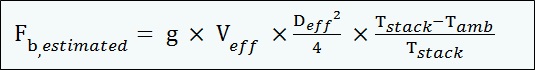
Setting Equation 4 and 5 equal to each other and rearranging and solving for Deff provides:
Equation 6:
Where:
- Deff
- effective diameter at the flame tip (m)
This approach for calculating Deff is widely used by many other regulatory agencies including the US EPA.
2.3 The Tiered Modelling Approach
This chapter builds on existing Ministry guidelines
A proponent may choose to go directly to a more refined approach to modelling emissions from open flares and skip any of the more conservative tiers. In some situations, for example, for facilities with existing issues, the Ministry may require a proponent to proceed directly to a more refined approach. However, it is important that the method for modelling open flares follows the calculation methodology described in this Technical Bulletin to ensure consistency among all facilities.
As outlined in ADMGO, modelling may be first undertaken with an approved screening model such as SCREEN3 that requires no meteorological inputs and has a built-in flare source type. As mentioned previously, if SCREEN3 is used, the model automatically determines screening pseudo-parameters. The flare source type must be used when using SCREEN3 to model flares (i.e. the use of calculated flare pseudo-parameters with the point source option in SCREEN3 is not permitted). Also note that SCREEN3 only considers one source at a time. If multiple emission sources are in operation during the flaring event, each source must be run individually and the maximum POI concentrations from each conservatively added to determine the total POI.
If this SCREEN3 modelling shows that the O. Reg. 419/05 air standards and guidelines will be met at all locations within the modelling domain, no further assessment is necessary. In cases where the O. Reg. 419/05 air standard or guideline is not met when using SCREEN3, then the proponent may use a more refined approach using an approved version of the AERMOD model (section 6 of O. Reg. 419/05), using a point source and the calculated effective pseudo-parameters. As well, as per the ADMGO, the appropriate regional meteorological data set may be used, or, if approved under subsection 13(1) of O. Reg. 419/05, a site-specific meteorological data
If refined modelling still shows an exceedence of a standard or guideline, then notification under section 28 of O. Reg. 419/05 is required.
2.4 Use of Alternate Approaches
Facilities that would like to further refine their assessments by incorporating additional site-specific elements (e.g. use of hourly variations in flame tilt, use of steam or air assist, etc.), into pseudo-parameter calculations can request a notice under section 13.1 of O. Reg. 419/05 in relation to determining the value of dispersion modelling parameters. Such requests must include the rationale for the approach, the information to be used, and the specific calculations or sample calculations to support the request.
References
AERFlare spreadsheet and User’s Guide – Alberta Environment Regulatory Flare Methodology (version 2.03).
Beychok, 1979. Fundamentals of Stack Gas Dispersion.
Leahey and Davies, 1984. Observations of Plume Rise from Sour Gas Flares. Atmospheric Env., Vol 18. No.5, pp 917-922.
San Joaquin Valley Air Pollution Control District – Flare Modelling Parameter Estimator Spreadsheet and user guidance.
Tan, 1967. Flare System Design Simplified. Hydrocarbon Processing. pp 172-176.
TCEQ, 2004. Technical Basis for Flare Parameters.
US EPA, 2012. Parameters for Properly Designed and Operated Flares. Report for Flare Review Panel. Office of Air Quality Planning and Standards (OAQPS). April.
This Bulletin is provided for information purposes only and should not be used to interpret any policy of the Ministry of the Environment and Climate Change (Ministry) nor any statute, regulation or other law. Further, this Bulletin does not provide any advice or permission in respect of any statute, regulation or law, nor does this Bulletin relieve any user from compliance with any statute, regulation or other law. The Ministry makes no warranty respecting the accuracy of the information contained in this Bulletin. Any use or application of the information contained in this Bulletin is at the sole risk of the user. The Ministry assumes no liability for any damages or other loss or injury which may result from the use or application of information contained in this Bulletin.
Appendix A - Sample Calculations
The sample calculations included in this appendix are for illustrative purposes only and meant to provide general guidance (e.g. they are not meant to represent an actual operating scenario). Actual project information may be different and more detailed supporting documentation may be required. Note that some calculations may not produce the exact results due to rounding errors.
Two streams are simultaneously sent to the flare at different flow rates and compositions. Natural gas is added to aid combustion and add “lift”. The individual stream compositions and total flared gas stream composition, molecular weight and flow rates are shown in Table A-1 below.
| Parameter | Unit | Stream 1 | Stream 2 | Natural Gas | Total Max to Flare |
|---|---|---|---|---|---|
| Mass Rate to Flare | kg/hr | 6800 | 2100 | 3250 | 12150 |
| Stream MW | kg/kgmol | 25.4 | 30.4 | 16.5 | 22.8 |
| Molar Weight to Flare | kgmol/hr | 268 | 69 | 197 | 534 |
| Volumetric Rate to Flare | m3/hr | 6429 | 1657 | 4742 | 12827 |
| Contaminant | Molecular Weight | Stream 1 | Stream 2 | Natural Gas | Total Max to Flare | |||||||||
|---|---|---|---|---|---|---|---|---|---|---|---|---|---|---|
| mol fraction | Flow Rate (kgmol/s) | Stream Emission Rate (g/s) | mol fraction | Flow Rate (kgmol/s) | Stream Emission Rate (g/s) | mol fraction | Flow Rate (kgmol/s) | Stream Emission Rate (g/s) | Emission Rate to Flare (g/s) | Emission Rate to Flare (mol/s) | mol fraction | Emission Rate From Flare (g/s) | ||
| Methane | 16.0 | 8.7E-01 | 6.4E-02 | 1032.8 | 4.0E-03 | 7.6E-05 | 1.2 | 9.7E-01 | 5.3E-02 | 848.9 | 1882.9 | 117.4 | 7.9E-01 | 56.5 |
| Ethane | 30.1 | 6.0E-03 | 4.5E-04 | 13.4 | 9.9E-01 | 1.9E-02 | 568.7 | 2.9E-02 | 1.6E-03 | 47.4 | 629.5 | 20.9 | 1.4E-01 | 18.9 |
| Propane | 44.1 | 1.9E-04 | 3.7E-06 | 0.2 | 1.6E-03 | 8.9E-05 | 3.9 | 4.1 | 0.09 | 6.3E-04 | 0.12 | |||
| n-Butane | 58.1 | 3.9E-04 | 2.1E-05 | 1.2 | 1.2 | 0.02 | 1.4E-04 | 0.04 | ||||||
| n-Pentane | 72.1 | 1.4E-04 | 7.7E-06 | 0.6 | 0.6 | 0.01 | 5.2E-05 | 0.02 | ||||||
| n-Hexane | 86.2 | 1.6E-04 | 8.8E-06 | 0.8 | 0.8 | 0.01 | 5.9-E05 | 0.02 | ||||||
| Benzene | 78.1 | 5.3E-02 | 3.9E-03 | 307.2 | 307.2 | 3.9 | 2.7E-02 | 9.2 | ||||||
| Toluene | 92.1 | 2.6E-02 | 1.9E-03 | 176.1 | 176.1 | 1.9 | 1.3E-02 | 5.3 | ||||||
| Ethyl benzene | 106.2 | 4.2E-02 | 3.1E-03 | 333.9 | 3.3E-04 | 6.3E-06 | 0.7 | 334.6 | 3.2 | 21.E-02 | 10 | |||
| Styrene | 104.2 | 3.3E-03 | 2.5E-04 | 25.6 | 25.6 | 0.25 | 1.7E-03 | 0.77 | ||||||
| 1,3 Diethylbenzene | 134.2 | 3.2E-03 | 6.1E-05 | 8.2 | 8.2 | 0.06 | 4.1E-04 | 0.25 | ||||||
| Light non-aromatics | 79.0 | 2.1E-03 | 4.1E-05 | 3.2 | 3.2 | 0.04 | 2.8E-04 | 0.10 | ||||||
| s-Butylbenzene | 134.0 | 4.8E-04 | 9.1E-06 | 1.2 | 1.2 | 0.01 | 6.2E-05 | 0.04 | ||||||
Note: Emission rates (ER) from the flare were calculated assuming 97% destruction efficiency in the flare.
This composition is used to calculate the Total Heat Release Rate (QT), to the flare as per Table A-2 below.
| Parameter | Value | Units |
|---|---|---|
| Mass Rate to Flare | 12150 | kg/hr |
| Stream MW | 22.8 | kg/kgmol |
| Molar Rate to Flare | 534 | kgmol/hr |
| Site Elevation | 195 | m |
| Site Atmospheric Pressure | 101.15 | kPa |
| Universal Gas Constant (R) | 8.3145 | (kPa-m3)/(K-kgmol) |
| Gas Temperature (Tgas) | 20 | °C |
| Gas Temperature (Tgas) | 293 | K |
| Volumetric Rate to Flare | 12827 | m3/hr |
| Specific Volume at actual conditions | 24.02 | m3/kgmol |
| Lower Explosive Limit | 4.5 | % |
| Total Heat Release Rate | 163.7 | MJ/s |
| Contaminant | Emission Rate to Flare (g/s) | Emission Rate to Flare (mol/s) | Emission Rate to Flare (m3/s) | mol fraction | LEL (%) | Fraction LEL | Lower Heating Value (MJ/m3) | Heat Release (MJ/s) |
|---|---|---|---|---|---|---|---|---|
| Methane | 1882.9 | 117.4 | 2.8E+00 | 7.9E-01 | 5.0 | 4.0E+00 | 34.0 | 96.2 |
| Ethane | 629.5 | 20.9 | 5.0E-01 | 1.4E-01 | 3.0 | 4.2E-01 | 61.1 | 30.8 |
| Propane | 4.1 | 0.09 | 2.2E-03 | 6.3E-04 | 2.1 | 1.3E-03 | 88.8 | 0.2 |
| n-Butane | 1.2 | 0.02 | 5.2E-04 | 1.4E-04 | 1.8 | 2.6E-04 | 116.2 | 0.1 |
| n-Pentane | 0.6 | 0.01 | 1.9E-04 | 5.2E-05 | 1.4 | 7.3E-05 | 138.2 | 0.0 |
| n-Hexane | 0.8 | 0.01 | 2.1E-04 | 5.9E-05 | 1.2 | 7.1E-05 | 138.2 | 0.0 |
| Benzene | 307.2 | 3.9 | 9.5E-02 | 2.7E-02 | 1.2 | 3.2E-02 | 133.8 | 12.7 |
| Toluene | 176.1 | 1.9 | 4.6E-02 | 1.3E-02 | 1.2 | 1.6E-02 | 156.7 | 7.2 |
| Ethyl Benzene | 334.6 | 3.2 | 7.6E-02 | 2.1E-02 | 1.0 | 2.1E-02 | 194.0 | 14.7 |
| Styrene | 25.6 | 0.25 | 5.9E-03 | 1.7E-03 | 0.9 | 1.5E-03 | 194.0 | 1.1 |
| 1,3 DEB | 8.2 | 0.06 | 1.5E-03 | 4.1E-04 | 0.8 | 3.3E-04 | 254.0 | 0.4 |
| Light non aromatics | 3.2 | 0.04 | 9.8E-04 | 2.8E-04 | 1.0 | 2.8E-04 | 133.8 | 0.1 |
| s-Butylbenzene | 1.2 | 0.01 | 2.2E-04 | 6.2E-05 | 0.8 | 4.9E-05 | 230.0 | 0.1 |
The molecular weight of the flared gas stream is 22.8 kg/kgmol. Based on this MW, a value of ƒ = 30% is selected from Table 1. Also, the LEL of the gas stream to be flared is 4.5%, which is less than the 15.3% value recommended by the US EPA to maintain good combustion. The MW and LEL were recalculated without the addition of natural gas, and were found to be 26.5 kg/kgmol and 4.2%, respectively, which are similar to the values that were calculated with the natural gas lift (i.e. this would not change the selected ƒ value).
The reference values to be used in the subsequent calculations are shown below in Table A-3.
| Parameter | Total Maximum to Flare (all 3 streams) Value | Total Maximum to Flare (all 3 streams) Units |
|---|---|---|
| Complete Combustion Total Heat Release Rate (QT) | 163.7 | MJ/s |
| Complete Combustion Total Heat Release Rate (QT) | 1.637E+08 | J/s |
| Flame Radiation Loss (ƒ) | 30 | % |
| Flame Radiation Loss (ƒ) | 0.3 | fraction |
| Flare Stack Tip Height (Hs) | 47 | m |
| Volumetric Rate to Flare (20°C, 101.15kPa) | 12827 | m3/hr |
| Volumetric Rate to Flare (20°C, 101.15kPa) | 3.56 | m3/s |
| Flare Stack Tip Diameter (Dnozzle) | 0.17 | m |
| Density of Flared Gas (ρgas) | 0.946 | kg/m3 |
| Density of Ambient Air at Ambient Air Temperature (ρair) | 1.183 | kg/m3 |
| Gravitational Constant (g) | 9.807 | m/s2 |
| Air Specific Heat at Ambient Air Temperature (Cp, air) | 1004 | J/(kg-K) |
| Modelled Ambient Air Temperature (Tair) | 25 | °C |
| Modelled Ambient Air Temperature (Tair) | 298 | K |
| Assumed Stack Gas Exit Temperature (Tstack) | 1273 | K |
The calculations for net heat release rate and effective stack height are as follows, based on Equation (1):

Based on the gas flow rate to the flare, and the nozzle diameter, the nozzle velocity is as follows:
The momentum flux is calculated as follows, based on Equation (2):
The buoyancy flux is calculated as follows, based on Equation (4):
The effective exit velocity is calculated as follows, based on Equation (3):
Finally, the effective diameter is calculated as follows, based on Equation (6):
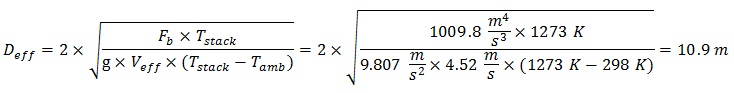
As a reminder, Veff and Deff are the effective values of velocity and diameter, respectively, at the flame tip.
Footnotes
- footnote[1] Back to paragraph A reference to an advanced dispersion model in this bulletin is a reference to AERMOD or another air dispersion model capable of using hourly meteorological observations to calculate contaminant dispersion and resulting POI concentrations if the model is approved under O. Reg. 419/05.
- footnote[2] Back to paragraph Note that the US EPA recommends that the Lower Explosive Limit (LEL) of a flared gas stream be 15.3 percent by volume or less to maintain good combustion efficiency (US EPA, 2012).
- footnote[3] Back to paragraph Alberta Environment formally revised its methodology in 2013.
- footnote[4] Back to paragraph Density at actual flare gas temperature and pressure at the nozzle (i.e., prior to combustion).
- footnote[5] Back to paragraph Density of air at ambient temperature and pressure.
- footnote[6] Back to paragraph Corrected to actual gas temperature and pressure.
- footnote[7] Back to paragraph “Procedure for Preparing an Emission Summary and Dispersion Modelling (ESDM) Report” (PIBs # 3614e04) (as amended).
- footnote[8] Back to paragraph “Air Dispersion Modelling Guideline for Ontario (ADMGO)” (PIBs # 5165e) (as amended).
- footnote[9] Back to paragraph MOECC Form Request for Approval under s. 13(1) of Regulation 419/05, for use of Site Specific Meteorological Data. (PIBs # 5350e).
- footnote[10] Back to paragraph MOE Form: Request under s. 7(1) of Regulation 419 for Use of a Specified Dispersion Model (PIBs # 5352e).