2018 default emission factors
1. Introduction
In April 2015, the province of Ontario announced its decision to establish a cap and trade program to reduce greenhouse gas (GHG) emissions. Importers of electricity into Ontario will be required to achieve compliance for the electricity they import under the program. Requiring imports to comply achieves two objectives, it:
- Levels the playing field between imported and domestically produced electricity; and
- Mitigates emissions leakage, which occurs when there is an increase in emissions in one jurisdiction because of a decrease in emissions in another jurisdiction, in this case Ontario.
Ontario established default emission factors annually for imported electricity from select jurisdictions in Canada and the US.
Navigant has developed a methodology for the Ontario Ministry of Energy to establish the default emission factors for the peak and off-peak periods for 2018 based on the emission intensity of marginal generation resources in the following key jurisdictions. The analysis also establishes a generic default emission factor for imports originating elsewhere:
- ISO-NE;
- NYISO;
- PJM;
- MISO; and
- Manitoba.
In October 2017, Navigant was retained to conduct analyses to determine default emission factors for 2018 using this methodology.
| Jurisdiction | Off Peak | Peak |
|---|---|---|
| ISO-NE | 0.297 | 0.414 |
| NYISO | 0.311 | 0.434 |
| PJM | 0.607 | 0.754 |
| MISO | 0.730 | 0.768 |
| Manitoba | 0 | 0 |
| Unspecified | 0.600 | 0.750 |
This report contains four sections and five appendices. The first section provides an introduction and describes the scope of Navigant’s work. The second section, describes the methodology to calculate the marginal default emission factors. The third section, discusses the sensitivity analysis that Navigant conducted on three aspects of the methodology. The fourth and final section presents the results of the methodology and the default emission factors. The appendices provide an overview of Navigant’s approach to electricity and natural gas market modelling for North America and the underlying assumptions for each jurisdiction.
2. Methodology
Through the use of marginal default emission factors, Ontario aims to minimize emission leakage and to create an efficient price signal for imports into Ontario relative to domestic production. The broad goal of the approach is to estimate the emissions of the marginal resource in the other jurisdictions that would provide replacement energy to make up for the energy that Ontario is importing in each time period – hence increasing GHG emissions in region that Ontario is importing from. This is valuable as an estimate of the magnitude of the emissions leakage from Ontario’s import from a specific region.
The general concept of a marginal resource is well-defined – the next available unit of production required to meet the next unit of demand. However, in the context of an electricity system managed through a security-constrained least cost dispatch, there are different ways to interpret, and determine, the marginal resource(s). Navigant also recognizes that there are different approaches that Ontario could take to estimate the emissions associated with imported electricity into Ontario.
Navigant’s approach relies on a mapping of a forecast of hourly locational marginal prices, averaged across nodes and zones to a single price for each jurisdiction, and the firing costs (i.e. the fuel and variable operating cost) of individual generating units within a jurisdiction to determine the marginal resource(s) in each hour. Once the marginal resource(s) are identified, a single emission intensity is then calculated for each hour and averaged across time periods to determine the default emission factors. This methodology is described in detail below.
2.1 Overview
The following six steps summarise Navigant’s methodology. Each step is described in further detail in the sections that follow.
- Using PROMOD, an industry-standard power market model, Navigant forecast unit dispatch and locational marginal prices within the entire Eastern Interconnection for 2018.
- Calculated a single hourly marginal price for each jurisdiction by calculating a load-weighted average of the hourly locational marginal prices for each node within each jurisdiction.
- Calculated the hourly firing cost (i.e. fuel and variable operating costs) for each generation unit within a jurisdiction.
- Grouped the generation units within each jurisdiction into deciles, based on firing cost, and calculated a capacity-weighted average emission intensity of the generation units within each decile.
- For each jurisdiction, mapped the hourly marginal price to the closest decile and assigned the emission intensity of that decile to the hour.
- Calculate the default emission factor for each jurisdiction by time period by averaging the assigned emission intensities for each hour by season and time of day, as appropriate.
2.2 Detailed Methodology
2.2.1 Forecast dispatch and price
Navigant used PROMOD to simulate the dispatch of the Eastern Interconnection and to forecast locational marginal prices. Appendix A contains more detail on Navigant’s approach to electricity market modelling in North America.
For the purpose of establishing the 2018 default emission factors, Navigant used PROMOD results from its Summer 2017 Reference Case to develop forward looking assumptions for 2018
2.2.2 Single price for each jurisdiction
PROMOD is a detailed hourly chronological market model that simulates the dispatch and operation of wholesale electricity markets. PROMOD can be run as a zonal or nodal model. Navigant runs it in the full nodal mode with full transmission representation, as opposed to a zonal model that aggregates transmission constraints. The nodal model establishes individual locational marginal prices for each generation node and a load-weighted locational marginal price for each zone and incorporates price drivers such as transmission congestion.
Figure 1 shows a graphical representation of the Electric Reliability Council of Texas (ERCOT) when viewed from a zonal and nodal perspective. While ERCOT is not part of this study, the figure provides a good comparison of the zonal and nodal views of a jurisdiction.
Figure 1. Illustration of Zones (left) and Nodes (right) in a Jurisdiction

Source: ERCOT. Press release regarding ERCOT change from zonal to nodal.
To establish a single price for each jurisdiction in every hour, Navigant calculated the load-weighted average of the individual zonal prices.
2.2.3 Calculation of firing costs and emission factor
Navigant calculated the firing cost per megawatt-hour for each generation unit using the following formula:
Hourly Firing Cost = (Fuel Cost x Heat Rate) + Variable O&M + Emissions Cost
The fuel costs vary by month
Emissions Cost = Emission Price * (Heat Rate x GHG Content of the Fuel)
For generation units that are subject to the Regional Greenhouse Gas Initiative (RGGI), Navigant assumed a price of USD 2016 $3.79 per metric tonne. GHG Content of the Fuel refers to the amount of carbon dioxide that is emitted when a million British Thermal Units (MMBtu) of fuel is combusted. The assumed carbon content of coal, oil and gas are 100.0, 77.3 and 54.1 kg per MMBtu respectively.
2.2.4 Emission factor by decil
Navigant grouped generation units within each jurisdiction into deciles by cumulative available capacity, such that each decile contains roughly the same amount of available generation. The first decile comprised the least expensive units and the tenth decile comprised the most expensive units. Navigant then calculated a single firing cost and emission intensity for each decile based on the capacity-weighted average firing cost and emission intensity of the generation units within each decile.
An example of the decile groupings for NYISO is presented in Figure 2. In general, renewable, hydro, and nuclear resources have the lowest firing cost in each region. This is followed by efficient gas units and coal units. The units with the highest firing cost are less efficient gas, coal, and oil fired units.
Figure 2. NYISO Decile Grouping
| Decile | Firing Cost | Emission Factor |
|---|---|---|
| 1 | $0.00 | 0.00 |
| 2 | $0.66 | 0.00 |
| 3 | $9.73 | 0.22 |
| 4 | $60.38 | 0.36 |
| 5 | $62.75 | 0.38 |
| 6 | $63.80 | 0.38 |
| 7 | $68.65 | 0.41 |
| 8 | $81.31 | 0.49 |
| 9 | $98.78 | 0.72 |
| 10 | $140.40 | 0.84 |
2.2.5 Map emission intensities to hourly prices
Navigant mapped an emission intensity to each hour of the year based on the emission intensity of the decile with the firing cost closest to the hourly price.
2.2.6 Default emission factors
Navigant calculated two annual default emission factors for each jurisdiction by averaging the hourly emission intensities across the peak and off-peak periods. Navigant used a non-standard definition of peak, 7:00 am eastern standard time to 10:59:59 pm eastern standard time seven days a week including holidays. Analysis supporting this definition of peak is contained in Section 3.2.
The choice of a single set of peak and off-peak factors, rather than multiple factors for each month or season, and the non-standard peak definition are discussed in more detail in Section 3.
2.2.7 Manitoba
The methodology outlined above was applied to all of the US jurisdictions. Manitoba, however, has a significantly different electricity system. Manitoba’s electricity comes almost entirely from renewable sources (hydroelectric and wind), and while there are some natural gas and one coal-fired generation unit, they are primarily dispatched for local reliability reasons and not for export.
Figure 3. Manitoba 2015 Installed Generation Capacity
| Category | % of supply |
|---|---|
| Renewable | 92% |
| Gas | 7% |
| Nuclear | 0% |
| Oil | 0% |
| Coal | 2% |
The renewable generation facilities in Manitoba have a marginal emission intensity of zero. Hence, similar to 2017, Navigant recommends that the default emission factors for 2018 for Manitoba be set at zero.
2.3 Generic factor
In addition to the default emission factors for specifically named jurisdictions, Navigant was retained to develop a methodology and propose default emission factors for imports emanating from other unspecified regions.
The vast majority of Ontario’s electricity imports originate in the specifically named jurisdictions. However, a very small number of imports in the past have originated in other parts of the Eastern Interconnection. Ontario does not import electricity from the Western Electricity Coordinating Council (WECC) or the Electricity Reliability Council of Texas (ERCOT).
Hence, to establish a generic factor for imports from the unspecified regions, Navigant compared the generation resource mix in the remainder of the Eastern Interconnection (i.e. excluding NYISO, MISO, PJM, ISO-NE, Manitoba and Ontario) to the specified jurisdictions.
Navigant found that the resource mix across the unspecified regions is similar to that of PJM. Thus, Navigant expects that if the marginal analysis was conducted for the reminder of the Eastern Interconnection, the results would be similar to PJM. As a result, Navigant recommends using the PJM default factors as the default factors for imports from any other jurisdiction.
Figure 4. Installed Capacity for Remainder of Eastern Interconnection and PJM
| Category | Remainder of Eastern Interconnect |
|---|---|
| Renewable | 18% |
| Gas | 41% |
| Nuclear | 10% |
| Oil | 4% |
| Coal | 27% |
| Category | PJM |
|---|---|
| Renewable | 12% |
| Gas | 34% |
| Nuclear | 18% |
| Oil | 5% |
| Coal | 31% |
3. Sensitivities and other considerations
Through the course of the analysis, Navigant identified several methodological assumptions that could have a material impact on the results. This section discusses the results of a sensitivity analysis around three such assumptions:
- The choice of a single factor for peak and off peak regardless of month or season;
- The choice of a non-standard peak definition; and
- The decision to include all zones and generation units within a jurisdiction, regardless of the historical pattern of power flows.
3.1 Seasons
The results presented in Section 4 are based on a single peak and off peak definition across the entire year. In other words, they do not vary materially by month or season. To understand the impact and validity of this assumption, Navigant analysed the pattern of average daily emissions by month and grouped them by season. The seasonal definitions are summarised in Table 2.
Table 2. Season Definitions
| Season | Months |
|---|---|
| Summer | May – August |
| Winter | November – December January – February |
| Shoulder | March – April September – October |
Navigant plotted the average daily emission factors for each jurisdiction by month, grouped by season, in order to identify similar patterns. Ultimately, Navigant concluded that, while some seasonal patterns exist, they were not strong enough within jurisdictions or consistent enough across jurisdictions to warrant seasonal emission factors.
For ISO-NE (Figure 5):
- There is little discernable pattern across the shoulder months;
- Across the summer and winter months the pattern is relatively consistent;
- Within the summer and winter periods there is considerable variability in the magnitude of the emission intensity; and
- The lowest average emission factor occurs in October (0.31), whereas the highest occurs in November (0.43).
| Month | Monday | Tuesday | Wednesday | Thursday | Friday | Saturday | Sunday |
|---|---|---|---|---|---|---|---|
| January | 0.37 | 0.37 | 0.37 | 0.37 | 0.39 | 0.38 | 0.37 |
| February | 0.35 | 0.35 | 0.37 | 0.37 | 0.38 | 0.38 | 0.35 |
| March | 0.39 | 0.40 | 0.39 | 0.40 | 0.39 | 0.42 | 0.39 |
| April | 0.35 | 0.35 | 0.35 | 0.35 | 0.38 | 0.38 | 0.35 |
| May | 0.35 | 0.36 | 0.36 | 0.37 | 0.39 | 0.39 | 0.42 |
| June | 0.36 | 0.35 | 0.37 | 0.37 | 0.40 | 0.40 | 0.42 |
| July | 0.38 | 0.37 | 0.37 | 0.36 | 0.41 | 0.40 | 0.39 |
| August | 0.38 | 0.37 | 0.37 | 0.39 | 0.40 | 0.39 | 0.40 |
| September | 0.37 | 0.36 | 0.37 | 0.35 | 0.39 | 0.38 | 0.38 |
| October | 0.33 | 0.35 | 0.31 | 0.31 | 0.37 | 0.37 | 0.35 |
| November | 0.41 | 0.40 | 0.40 | 0.39 | 0.37 | 0.40 | 0.43 |
| December | 0.37 | 0.36 | 0.37 | 0.37 | 0.37 | 0.38 | 0.37 |
For NYISO (Figure 6):
- There is consistency across weekdays and weekends in all three seasons except for January and February in the winter;
- The summer period displays more variability in the magnitude of the emission intensity compared to the winter and shoulder periods;
- July is an outlier; and
- The lowest average emission factor occurs in September (0.31), whereas the highest occurs in July (0.50).
| Date | Monday | Tuesday | Wednesday | Thursday | Friday | Saturday | Sunday |
|---|---|---|---|---|---|---|---|
| January | 0.38 | 0.38 | 0.38 | 0.38 | 0.38 | 0.38 | 0.38 |
| February | 0.38 | 0.38 | 0.38 | 0.38 | 0.38 | 0.38 | 0.38 |
| March | 0.41 | 0.43 | 0.42 | 0.40 | 0.37 | 0.38 | 0.42 |
| April | 0.36 | 0.35 | 0.38 | 0.37 | 0.35 | 0.35 | 0.39 |
| May | 0.36 | 0.36 | 0.35 | 0.35 | 0.33 | 0.32 | 0.39 |
| June | 0.44 | 0.43 | 0.43 | 0.43 | 0.41 | 0.41 | 0.45 |
| July | 0.49 | 0.49 | 0.48 | 0.48 | 0.45 | 0.45 | 0.50 |
| August | 0.42 | 0.42 | 0.44 | 0.43 | 0.40 | 0.39 | 0.43 |
| September | 0.36 | 0.36 | 0.38 | 0.36 | 0.33 | 0.31 | 0.38 |
| October | 0.33 | 0.34 | 0.33 | 0.32 | 0.35 | 0.33 | 0.36 |
| November | 0.44 | 0.44 | 0.41 | 0.41 | 0.39 | 0.39 | 0.45 |
| December | 0.40 | 0.40 | 0.40 | 0.40 | 0.40 | 0.40 | 0.41 |
For PJM (Figure 7):
- Within the winter season the profiles are generally consistent with January and February having higher emission factors;
- The pattern in the shoulder months is distinctly different than the winter and shoulder;
- The end of the week and weekends in May are different from the remainder of the summer; and
- The lowest average emission factor occurs in March (0.58), whereas the highest occurs in February (0.82).
| Date | Monday | Tuesday | Wednesday | Thursday | Friday | Saturday | Sunday |
|---|---|---|---|---|---|---|---|
| January | 0.80 | 0.78 | 0.78 | 0.79 | 0.80 | 0.81 | 0.81 |
| February | 0.78 | 0.79 | 0.79 | 0.80 | 0.80 | 0.82 | 0.79 |
| March | 0.63 | 0.63 | 0.62 | 0.62 | 0.65 | 0.68 | 0.63 |
| April | 0.70 | 0.69 | 0.71 | 0.69 | 0.61 | 0.58 | 0.74 |
| May | 0.72 | 0.73 | 0.73 | 0.73 | 0.62 | 0.59 | 0.75 |
| June | 0.69 | 0.70 | 0.69 | 0.68 | 0.67 | 0.66 | 0.71 |
| July | 0.71 | 0.70 | 0.69 | 0.68 | 0.71 | 0.70 | 0.71 |
| August | 0.71 | 0.70 | 0.70 | 0.69 | 0.69 | 0.69 | 0.69 |
| September | 0.73 | 0.73 | 0.71 | 0.69 | 0.65 | 0.62 | 0.73 |
| October | 0.72 | 0.73 | 0.75 | 0.73 | 0.64 | 0.60 | 0.74 |
| November | 0.70 | 0.70 | 0.72 | 0.70 | 0.71 | 0.70 | 0.71 |
| December | 0.68 | 0.68 | 0.68 | 0.68 | 0.69 | 0.71 | 0.69 |
For MISO (Figure 8):
- Within the winter months the profiles are generally consistent;
- The shoulder months display more variability than the winter and shoulder;
- The end of the week and weekends in May are different from the remainder of the summer; and
- The lowest average emission factor occurs in April (0.69), whereas the highest occurs in December (0.81).
| Date | Monday | Tuesday | Wednesday | Thursday | Friday | Saturday | Sunday |
|---|---|---|---|---|---|---|---|
| January | 0.75 | 0.75 | 0.75 | 0.74 | 0.77 | 0.74 | 0.74 |
| February | 0.74 | 0.75 | 0.74 | 0.74 | 0.74 | 0.74 | 0.73 |
| March | 0.79 | 0.78 | 0.78 | 0.79 | 0.77 | 0.77 | 0.79 |
| April | 0.75 | 0.74 | 0.76 | 0.75 | 0.70 | 0.69 | 0.79 |
| May | 0.73 | 0.75 | 0.75 | 0.76 | 0.69 | 0.70 | 0.76 |
| June | 0.75 | 0.75 | 0.75 | 0.75 | 0.75 | 0.74 | 0.76 |
| July | 0.75 | 0.75 | 0.76 | 0.74 | 0.77 | 0.76 | 0.76 |
| August | 0.75 | 0.76 | 0.76 | 0.76 | 0.77 | 0.77 | 0.77 |
| September | 0.76 | 0.76 | 0.77 | 0.76 | 0.80 | 0.79 | 0.75 |
| October | 0.75 | 0.75 | 0.73 | 0.74 | 0.79 | 0.77 | 0.77 |
| November | 0.72 | 0.73 | 0.74 | 0.74 | 0.76 | 0.78 | 0.74 |
| December | 0.75 | 0.75 | 0.76 | 0.76 | 0.79 | 0.81 | 0.76 |
3.2 Peak period
The results presented in the Section 4 are based on a non-standard definition of the peak period. The decision to use a non-standard definition was based on an analysis of hourly emission factors within each jurisdiction.
Navigant analysed the pattern of hourly emission intensity for an average week in each jurisdiction. The graphs below show the profile of hourly emission intensities starting on a Monday at 12:00 am Eastern Standard Time through to Sunday evening at 11:59:59 pm.
As observed for 2017, the charts below for 2018 show that the emission intensity during the daytime on weekends more closely resembles the emission intensity during the daytime on weekdays. As a result, Navigant recommended using the non-standard definition for 2018 which is based on a 16 hour-per day peak period seven days a week, rather than the standard five days a week definition typically used by the Independent System Operators. Navigant believes that this definition results in a more uniform emission factor within each period.
| Hour of the Week |
DEF |
|---|---|
| 1 | 0.22 |
| 2 | 0.18 |
| 3 | 0.21 |
| 4 | 0.19 |
| 5 | 0.27 |
| 6 | 0.37 |
| 7 | 0.40 |
| 8 | 0.42 |
| 9 | 0.43 |
| 10 | 0.43 |
| 11 | 0.43 |
| 12 | 0.43 |
| 13 | 0.41 |
| 14 | 0.40 |
| 15 | 0.40 |
| 16 | 0.40 |
| 17 | 0.42 |
| 18 | 0.43 |
| 19 | 0.45 |
| 20 | 0.43 |
| 21 | 0.40 |
| 22 | 0.38 |
| 23 | 0.36 |
| 24 | 0.32 |
| 25 | 0.19 |
| 26 | 0.19 |
| 27 | 0.17 |
| 28 | 0.19 |
| 29 | 0.24 |
| 30 | 0.37 |
| 31 | 0.40 |
| 32 | 0.41 |
| 33 | 0.43 |
| 34 | 0.44 |
| 35 | 0.43 |
| 36 | 0.42 |
| 37 | 0.41 |
| 38 | 0.40 |
| 39 | 0.40 |
| 40 | 0.41 |
| 41 | 0.42 |
| 42 | 0.44 |
| 43 | 0.45 |
| 44 | 0.44 |
| 45 | 0.42 |
| 46 | 0.38 |
| 47 | 0.36 |
| 48 | 0.32 |
| 49 | 0.24 |
| 50 | 0.18 |
| 51 | 0.19 |
| 52 | 0.22 |
| 53 | 0.27 |
| 54 | 0.36 |
| 55 | 0.40 |
| 56 | 0.42 |
| 57 | 0.41 |
| 58 | 0.43 |
| 59 | 0.43 |
| 60 | 0.42 |
| 61 | 0.41 |
| 62 | 0.41 |
| 63 | 0.40 |
| 64 | 0.41 |
| 65 | 0.42 |
| 66 | 0.44 |
| 67 | 0.45 |
| 68 | 0.43 |
| 69 | 0.41 |
| 70 | 0.38 |
| 71 | 0.37 |
| 72 | 0.31 |
| 73 | 0.23 |
| 74 | 0.20 |
| 75 | 0.18 |
| 76 | 0.22 |
| 77 | 0.25 |
| 78 | 0.37 |
| 79 | 0.39 |
| 80 | 0.40 |
| 81 | 0.42 |
| 82 | 0.43 |
| 83 | 0.44 |
| 84 | 0.44 |
| 85 | 0.42 |
| 86 | 0.41 |
| 87 | 0.41 |
| 88 | 0.42 |
| 89 | 0.43 |
| 90 | 0.44 |
| 91 | 0.44 |
| 92 | 0.43 |
| 93 | 0.41 |
| 94 | 0.37 |
| 95 | 0.35 |
| 96 | 0.33 |
| 97 | 0.34 |
| 98 | 0.31 |
| 99 | 0.30 |
| 100 | 0.32 |
| 101 | 0.32 |
| 102 | 0.36 |
| 103 | 0.37 |
| 104 | 0.38 |
| 105 | 0.39 |
| 106 | 0.40 |
| 107 | 0.41 |
| 108 | 0.40 |
| 109 | 0.39 |
| 110 | 0.40 |
| 111 | 0.40 |
| 112 | 0.40 |
| 113 | 0.43 |
| 114 | 0.51 |
| 115 | 0.48 |
| 116 | 0.45 |
| 117 | 0.42 |
| 118 | 0.37 |
| 119 | 0.36 |
| 120 | 0.35 |
| 121 | 0.34 |
| 122 | 0.36 |
| 123 | 0.35 |
| 124 | 0.35 |
| 125 | 0.37 |
| 126 | 0.35 |
| 127 | 0.38 |
| 128 | 0.36 |
| 129 | 0.37 |
| 130 | 0.38 |
| 131 | 0.38 |
| 132 | 0.38 |
| 133 | 0.38 |
| 134 | 0.38 |
| 135 | 0.38 |
| 136 | 0.39 |
| 137 | 0.42 |
| 138 | 0.51 |
| 139 | 0.50 |
| 140 | 0.46 |
| 141 | 0.42 |
| 142 | 0.39 |
| 143 | 0.37 |
| 144 | 0.34 |
| 145 | 0.30 |
| 146 | 0.26 |
| 147 | 0.29 |
| 148 | 0.30 |
| 149 | 0.30 |
| 150 | 0.38 |
| 151 | 0.40 |
| 152 | 0.41 |
| 153 | 0.42 |
| 154 | 0.42 |
| 155 | 0.43 |
| 156 | 0.43 |
| 157 | 0.42 |
| 158 | 0.41 |
| 159 | 0.41 |
| 160 | 0.41 |
| 161 | 0.41 |
| 162 | 0.45 |
| 163 | 0.45 |
| 164 | 0.44 |
| 165 | 0.42 |
| 166 | 0.39 |
| 167 | 0.37 |
| 168 | 0.32 |
| Hour of the Week |
DEF |
|---|---|
| 1 | 0.27 |
| 2 | 0.28 |
| 3 | 0.26 |
| 4 | 0.26 |
| 5 | 0.29 |
| 6 | 0.35 |
| 7 | 0.43 |
| 8 | 0.45 |
| 9 | 0.46 |
| 10 | 0.47 |
| 11 | 0.47 |
| 12 | 0.46 |
| 13 | 0.43 |
| 14 | 0.42 |
| 15 | 0.43 |
| 16 | 0.43 |
| 17 | 0.47 |
| 18 | 0.47 |
| 19 | 0.47 |
| 20 | 0.46 |
| 21 | 0.44 |
| 22 | 0.42 |
| 23 | 0.36 |
| 24 | 0.31 |
| 25 | 0.27 |
| 26 | 0.28 |
| 27 | 0.27 |
| 28 | 0.29 |
| 29 | 0.29 |
| 30 | 0.35 |
| 31 | 0.42 |
| 32 | 0.45 |
| 33 | 0.47 |
| 34 | 0.46 |
| 35 | 0.46 |
| 36 | 0.45 |
| 37 | 0.43 |
| 38 | 0.43 |
| 39 | 0.42 |
| 40 | 0.44 |
| 41 | 0.46 |
| 42 | 0.46 |
| 43 | 0.46 |
| 44 | 0.46 |
| 45 | 0.44 |
| 46 | 0.41 |
| 47 | 0.36 |
| 48 | 0.31 |
| 49 | 0.28 |
| 50 | 0.28 |
| 51 | 0.28 |
| 52 | 0.28 |
| 53 | 0.30 |
| 54 | 0.34 |
| 55 | 0.42 |
| 56 | 0.45 |
| 57 | 0.45 |
| 58 | 0.46 |
| 59 | 0.46 |
| 60 | 0.45 |
| 61 | 0.43 |
| 62 | 0.42 |
| 63 | 0.43 |
| 64 | 0.44 |
| 65 | 0.46 |
| 66 | 0.47 |
| 67 | 0.47 |
| 68 | 0.46 |
| 69 | 0.44 |
| 70 | 0.42 |
| 71 | 0.35 |
| 72 | 0.30 |
| 73 | 0.29 |
| 74 | 0.27 |
| 75 | 0.26 |
| 76 | 0.28 |
| 77 | 0.29 |
| 78 | 0.35 |
| 79 | 0.42 |
| 80 | 0.44 |
| 81 | 0.45 |
| 82 | 0.46 |
| 83 | 0.46 |
| 84 | 0.45 |
| 85 | 0.44 |
| 86 | 0.42 |
| 87 | 0.42 |
| 88 | 0.44 |
| 89 | 0.46 |
| 90 | 0.47 |
| 91 | 0.46 |
| 92 | 0.46 |
| 93 | 0.45 |
| 94 | 0.39 |
| 95 | 0.33 |
| 96 | 0.30 |
| 97 | 0.32 |
| 98 | 0.29 |
| 99 | 0.29 |
| 100 | 0.29 |
| 101 | 0.29 |
| 102 | 0.30 |
| 103 | 0.34 |
| 104 | 0.35 |
| 105 | 0.39 |
| 106 | 0.41 |
| 107 | 0.41 |
| 108 | 0.41 |
| 109 | 0.39 |
| 110 | 0.39 |
| 111 | 0.39 |
| 112 | 0.40 |
| 113 | 0.45 |
| 114 | 0.49 |
| 115 | 0.50 |
| 116 | 0.48 |
| 117 | 0.45 |
| 118 | 0.39 |
| 119 | 0.33 |
| 120 | 0.31 |
| 121 | 0.31 |
| 122 | 0.30 |
| 123 | 0.31 |
| 124 | 0.30 |
| 125 | 0.30 |
| 126 | 0.31 |
| 127 | 0.32 |
| 128 | 0.34 |
| 129 | 0.34 |
| 130 | 0.36 |
| 131 | 0.37 |
| 132 | 0.37 |
| 133 | 0.38 |
| 134 | 0.37 |
| 135 | 0.38 |
| 136 | 0.39 |
| 137 | 0.44 |
| 138 | 0.50 |
| 139 | 0.51 |
| 140 | 0.50 |
| 141 | 0.45 |
| 142 | 0.42 |
| 143 | 0.37 |
| 144 | 0.33 |
| 145 | 0.30 |
| 146 | 0.31 |
| 147 | 0.30 |
| 148 | 0.31 |
| 149 | 0.32 |
| 150 | 0.37 |
| 151 | 0.43 |
| 152 | 0.46 |
| 153 | 0.46 |
| 154 | 0.47 |
| 155 | 0.48 |
| 156 | 0.45 |
| 157 | 0.43 |
| 158 | 0.44 |
| 159 | 0.43 |
| 160 | 0.45 |
| 161 | 0.47 |
| 162 | 0.49 |
| 163 | 0.47 |
| 164 | 0.47 |
| 165 | 0.47 |
| 166 | 0.42 |
| 167 | 0.36 |
| 168 | 0.31 |
| Hour of the Week |
DEF |
|---|---|
| 1 | 0.55 |
| 2 | 0.54 |
| 3 | 0.55 |
| 4 | 0.55 |
| 5 | 0.59 |
| 6 | 0.78 |
| 7 | 0.73 |
| 8 | 0.77 |
| 9 | 0.82 |
| 10 | 0.82 |
| 11 | 0.80 |
| 12 | 0.78 |
| 13 | 0.77 |
| 14 | 0.78 |
| 15 | 0.77 |
| 16 | 0.77 |
| 17 | 0.77 |
| 18 | 0.72 |
| 19 | 0.72 |
| 20 | 0.71 |
| 21 | 0.78 |
| 22 | 0.79 |
| 23 | 0.70 |
| 24 | 0.62 |
| 25 | 0.56 |
| 26 | 0.55 |
| 27 | 0.55 |
| 28 | 0.55 |
| 29 | 0.60 |
| 30 | 0.78 |
| 31 | 0.72 |
| 32 | 0.76 |
| 33 | 0.79 |
| 34 | 0.81 |
| 35 | 0.77 |
| 36 | 0.78 |
| 37 | 0.77 |
| 38 | 0.79 |
| 39 | 0.80 |
| 40 | 0.80 |
| 41 | 0.74 |
| 42 | 0.72 |
| 43 | 0.70 |
| 44 | 0.70 |
| 45 | 0.77 |
| 46 | 0.80 |
| 47 | 0.69 |
| 48 | 0.63 |
| 49 | 0.56 |
| 50 | 0.55 |
| 51 | 0.55 |
| 52 | 0.56 |
| 53 | 0.61 |
| 54 | 0.75 |
| 55 | 0.74 |
| 56 | 0.76 |
| 57 | 0.80 |
| 58 | 0.81 |
| 59 | 0.78 |
| 60 | 0.79 |
| 61 | 0.78 |
| 62 | 0.78 |
| 63 | 0.78 |
| 64 | 0.78 |
| 65 | 0.74 |
| 66 | 0.72 |
| 67 | 0.68 |
| 68 | 0.73 |
| 69 | 0.76 |
| 70 | 0.77 |
| 71 | 0.67 |
| 72 | 0.61 |
| 73 | 0.56 |
| 74 | 0.54 |
| 75 | 0.53 |
| 76 | 0.56 |
| 77 | 0.60 |
| 78 | 0.76 |
| 79 | 0.75 |
| 80 | 0.75 |
| 81 | 0.79 |
| 82 | 0.81 |
| 83 | 0.80 |
| 84 | 0.79 |
| 85 | 0.78 |
| 86 | 0.78 |
| 87 | 0.79 |
| 88 | 0.77 |
| 89 | 0.74 |
| 90 | 0.71 |
| 91 | 0.70 |
| 92 | 0.70 |
| 93 | 0.78 |
| 94 | 0.73 |
| 95 | 0.61 |
| 96 | 0.58 |
| 97 | 0.61 |
| 98 | 0.55 |
| 99 | 0.53 |
| 100 | 0.54 |
| 101 | 0.54 |
| 102 | 0.58 |
| 103 | 0.65 |
| 104 | 0.69 |
| 105 | 0.74 |
| 106 | 0.76 |
| 107 | 0.80 |
| 108 | 0.81 |
| 109 | 0.77 |
| 110 | 0.73 |
| 111 | 0.72 |
| 112 | 0.73 |
| 113 | 0.78 |
| 114 | 0.68 |
| 115 | 0.74 |
| 116 | 0.78 |
| 117 | 0.80 |
| 118 | 0.70 |
| 119 | 0.62 |
| 120 | 0.59 |
| 121 | 0.58 |
| 122 | 0.57 |
| 123 | 0.56 |
| 124 | 0.55 |
| 125 | 0.56 |
| 126 | 0.57 |
| 127 | 0.62 |
| 128 | 0.66 |
| 129 | 0.68 |
| 130 | 0.70 |
| 131 | 0.72 |
| 132 | 0.75 |
| 133 | 0.76 |
| 134 | 0.72 |
| 135 | 0.72 |
| 136 | 0.74 |
| 137 | 0.78 |
| 138 | 0.70 |
| 139 | 0.70 |
| 140 | 0.72 |
| 141 | 0.79 |
| 142 | 0.79 |
| 143 | 0.71 |
| 144 | 0.63 |
| 145 | 0.56 |
| 146 | 0.58 |
| 147 | 0.57 |
| 148 | 0.59 |
| 149 | 0.62 |
| 150 | 0.78 |
| 151 | 0.75 |
| 152 | 0.77 |
| 153 | 0.83 |
| 154 | 0.83 |
| 155 | 0.79 |
| 156 | 0.80 |
| 157 | 0.78 |
| 158 | 0.79 |
| 159 | 0.79 |
| 160 | 0.77 |
| 161 | 0.76 |
| 162 | 0.73 |
| 163 | 0.72 |
| 164 | 0.74 |
| 165 | 0.79 |
| 166 | 0.80 |
| 167 | 0.69 |
| 168 | 0.62 |
| Hour of the Week |
DEF |
|---|---|
| 1 | 0.69 |
| 2 | 0.68 |
| 3 | 0.68 |
| 4 | 0.70 |
| 5 | 0.76 |
| 6 | 0.80 |
| 7 | 0.78 |
| 8 | 0.78 |
| 9 | 0.79 |
| 10 | 0.78 |
| 11 | 0.76 |
| 12 | 0.75 |
| 13 | 0.74 |
| 14 | 0.74 |
| 15 | 0.74 |
| 16 | 0.74 |
| 17 | 0.75 |
| 18 | 0.74 |
| 19 | 0.75 |
| 20 | 0.76 |
| 21 | 0.77 |
| 22 | 0.80 |
| 23 | 0.75 |
| 24 | 0.74 |
| 25 | 0.72 |
| 26 | 0.71 |
| 27 | 0.70 |
| 28 | 0.72 |
| 29 | 0.76 |
| 30 | 0.81 |
| 31 | 0.78 |
| 32 | 0.78 |
| 33 | 0.78 |
| 34 | 0.77 |
| 35 | 0.76 |
| 36 | 0.76 |
| 37 | 0.74 |
| 38 | 0.74 |
| 39 | 0.74 |
| 40 | 0.74 |
| 41 | 0.74 |
| 42 | 0.74 |
| 43 | 0.75 |
| 44 | 0.74 |
| 45 | 0.77 |
| 46 | 0.80 |
| 47 | 0.78 |
| 48 | 0.74 |
| 49 | 0.72 |
| 50 | 0.70 |
| 51 | 0.69 |
| 52 | 0.71 |
| 53 | 0.76 |
| 54 | 0.81 |
| 55 | 0.77 |
| 56 | 0.78 |
| 57 | 0.78 |
| 58 | 0.77 |
| 59 | 0.77 |
| 60 | 0.75 |
| 61 | 0.75 |
| 62 | 0.75 |
| 63 | 0.75 |
| 64 | 0.75 |
| 65 | 0.75 |
| 66 | 0.76 |
| 67 | 0.75 |
| 68 | 0.75 |
| 69 | 0.76 |
| 70 | 0.82 |
| 71 | 0.77 |
| 72 | 0.74 |
| 73 | 0.71 |
| 74 | 0.70 |
| 75 | 0.67 |
| 76 | 0.68 |
| 77 | 0.73 |
| 78 | 0.82 |
| 79 | 0.79 |
| 80 | 0.79 |
| 81 | 0.79 |
| 82 | 0.77 |
| 83 | 0.77 |
| 84 | 0.76 |
| 85 | 0.75 |
| 86 | 0.74 |
| 87 | 0.75 |
| 88 | 0.75 |
| 89 | 0.75 |
| 90 | 0.75 |
| 91 | 0.75 |
| 92 | 0.75 |
| 93 | 0.77 |
| 94 | 0.79 |
| 95 | 0.75 |
| 96 | 0.75 |
| 97 | 0.74 |
| 98 | 0.69 |
| 99 | 0.65 |
| 100 | 0.67 |
| 101 | 0.69 |
| 102 | 0.72 |
| 103 | 0.75 |
| 104 | 0.79 |
| 105 | 0.81 |
| 106 | 0.81 |
| 107 | 0.81 |
| 108 | 0.81 |
| 109 | 0.80 |
| 110 | 0.80 |
| 111 | 0.79 |
| 112 | 0.80 |
| 113 | 0.77 |
| 114 | 0.74 |
| 115 | 0.76 |
| 116 | 0.79 |
| 117 | 0.80 |
| 118 | 0.78 |
| 119 | 0.74 |
| 120 | 0.73 |
| 121 | 0.73 |
| 122 | 0.71 |
| 123 | 0.69 |
| 124 | 0.67 |
| 125 | 0.69 |
| 126 | 0.71 |
| 127 | 0.74 |
| 128 | 0.78 |
| 129 | 0.78 |
| 130 | 0.77 |
| 131 | 0.79 |
| 132 | 0.79 |
| 133 | 0.79 |
| 134 | 0.78 |
| 135 | 0.79 |
| 136 | 0.79 |
| 137 | 0.77 |
| 138 | 0.74 |
| 139 | 0.76 |
| 140 | 0.76 |
| 141 | 0.80 |
| 142 | 0.79 |
| 143 | 0.77 |
| 144 | 0.77 |
| 145 | 0.75 |
| 146 | 0.73 |
| 147 | 0.72 |
| 148 | 0.74 |
| 149 | 0.78 |
| 150 | 0.82 |
| 151 | 0.78 |
| 152 | 0.77 |
| 153 | 0.77 |
| 154 | 0.77 |
| 155 | 0.77 |
| 156 | 0.76 |
| 157 | 0.75 |
| 158 | 0.75 |
| 159 | 0.75 |
| 160 | 0.75 |
| 161 | 0.76 |
| 162 | 0.76 |
| 163 | 0.76 |
| 164 | 0.76 |
| 165 | 0.77 |
| 166 | 0.80 |
| 167 | 0.75 |
| 168 | 0.74 |
3.3 Transmission constraints
Another methodological assumption that Navigant tested was the exclusion of highly congested zones from the calculation of the default emission factors.
From a practical standpoint, there are a number of zones within the specified jurisdictions that are transmission constrained and as a result are generally not the source of imports into Ontario (e.g., New York City). As such, an argument could be made that these zones should be excluded from the analysis.
To test this hypothesis and the impact on the results, Navigant ran the analysis for NYISO by excluding New York City and Long Island (zones J and K respectively) and for PJM by excluding zones in the transmission constrained east (JCPL, METED, OVEC, PECO, PENELEC, PEPCO, PPL, PSEG, RECO, UGI). In both cases, Navigant did not find materially differing results.
The specific zones selected for exclusion could be a matter of debate. Hence, based on the limited impact observed through the sensitivity analysis, Navigant recommends including all zones and generation units within a jurisdiction in the calculation of the emission factor for the jurisdiction.
3.4 Comparison with California and Quebec
Effective January 1, 2018 Ontario’s cap and trade program will be linked to the programs in California and Quebec. Therefore, it is important to understand how the emission factors for the Ontario program align with the emission factors used in California and Quebec.
For the most part, California uses specific emission factors tied to the specific generating resource from which the electricity is being imported. For the rare unspecified imports, California applies a default emission factor of 0.428 MTCO2e/MWh.
Similarly, where possible, Quebec applies an emission factor tied to the specific generating resource from with the electricity is being imported. For imports into Quebec that are sourced from an identifiable facility for which the information needed to calculate specific greenhouse gas emissions is not available, and for imports from unidentifiable facilities, Quebec relies on the following calculation and default regional factors.
GHG = MWhimp * EFD
Where:
- GHG = Annual greenhouse gas emissions attributable to the production of electricity acquired outside Québec and produced by the identifiable facility, in tonnes CO2 equivalent;
- MWhimp = Total quantity of electricity acquired from the identifiable facility and consumed or sold annually in Québec, including an estimate of transmission losses, from the facility’s busbar, in megawatt-hours;
- EFD = Greenhouse gas emission factor for the province or North American market from which the electricity comes, in tonnes of CO2 per megawatt-hour:
- As indicated in Table 3
footnote 6 ; - Zero when the electricity comes from an identifiable nuclear, hydroelectric, sea current, wind, solar or tidal power facility; and
- 0.999 if the electricity comes from a non-identifiable facility.
- As indicated in Table 3
| Jurisdiction | Default Emission Factor |
|---|---|
| Newfoundland and Labrador | 0.030 |
| Nova Scotia | 0.694 |
| New Brunswick | 0.292 |
| Québec | 0.002 |
| Ontario | 0.041 |
| Manitoba | 0.003 |
| Vermont | 0.002 |
| ISO-NE | 0.266 |
| NYISO | 0.242 |
| PJM | 0.592 |
| MISO | 0.638 |
| SPP | 0.614 |
4. Results
This section presents the results of the methodology outlined in Section 2 and Navigant’s default emission factors for 2018.
The key drivers that determine the emission factors for a region are:
- Relative prices of coal and gas – as gas becomes cheaper, it becomes economical to operate gas plants during the off-peak periods, as opposed to coal, as well as opposed to just the peak periods
footnote 8 ; - Various climate initiatives coupled with the declining costs curves for renewable technologies drives increases in renewable capacity in North America; and
- Coal retirements – less coal in the system will lower the overall emission factor for a region.
The table below shows the approximate emission factors for various fuels:
| Fuel | Emission Factor |
|---|---|
| Coal | 1.00 |
| Gas – Combustion Turbine | 0.65 |
| Gas – Combined Cycle | 0.40 |
| Renewables / Nuclear | 0.00 |
4.1 ISO specific factors
The calculated default emission factors for each jurisdiction are shown in the table below:
| Jurisdiction | Off Peak | Peak |
|---|---|---|
| ISO-NE | 0.297 | 0.414 |
| NYISO | 0.311 | 0.434 |
| PJM | 0.607 | 0.754 |
| MISO | 0.730 | 0.768 |
| Manitoba | 0.000 | 0.000 |
Within the U.S. jurisdictions under consideration, ISO-NE and NYISO have the lowest default emissions factors. Both regions have retired almost all their coal capacity and are expanding renewable generation and combined cycle gas capacity. This results in a mix of zero emission resources and combined cycle gas on the margin during off peak periods and combined cycle gas and some simple cycle gas on the margin during on peak periods.
PJM and MISO have significantly higher default emission factors due to significant coal generation and relatively less zero emission generation than the other two regions. In both regions, default emissions factors reflect the marginal resource being a mix of coal and gas generation in both peak and off peak times.
For Manitoba, a factor of zero is appropriate as discussed in Section 2.2.7.
4.2 Generic factor
As outlined in Section 2.3 Navigant recommends using the PJM results as the default factors for other, non-specified jurisdictions. The emission factors presented in Table 6 are rounded for simplicity.
| Jurisdiction | Off Peak | Peak |
|---|---|---|
| Unspecified | 0.600 | 0.750 |
Appendix A. Electricity market modelling methodology
Navigant employs a variety of commercial and proprietary energy market modeling tools to project generating capacity retirements and additions, generating unit dispatch, fuel consumption, gas pipeline flows, and commodity prices in organized (e.g., ISO-NE, NYISO, PJM, ERCOT, MISO, SPP, CA-ISO) and traditional markets (e.g., Southeast, Pacific Northwest). A schematic of these tools is shown below, followed by a brief description of each tool.
Figure 13. Navigant Energy Market Modeling Toolset
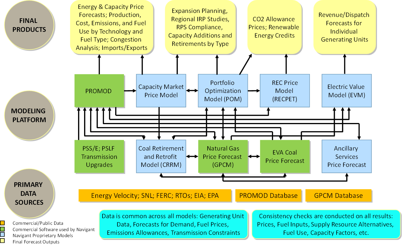
A.1 PROMOD Electric System Simulation Model
PROMOD IV is a detailed hourly chronological market model that simulates the dispatch and operation of the wholesale electricity market. This model replicates the least-cost optimization decision criteria used by system operators and utilities in the market while observing generating operational limitations and transmission constraints. PROMOD can be run as a zonal or nodal model; although Navigant normally runs it in the full nodal model with full transmission representation.
A.2 Transmission Planning – PSS/E, PSLF, and MUST
Both PSS/E and PSLF are transmission planning software licensed from Siemens PTI and GE, respectively. Both programs include power flow, optimal power flow, balanced and unbalanced fault analysis, dynamic simulations, extended term dynamic simulations, open access and pricing, transfer limit analysis, and network reduction. Siemens PTI's MUST is used to determine transmission transfer capability (FCITC, ATC, TTC) by simulating network conditions with equipment outages under different loading conditions.
A.3 Gas Price Competition Model (GPCM)
GPCM is a commercial linear-programming model of the North American gas marketplace and infrastructure. Navigant applies its own analysis to provide macroeconomic outlook and natural gas supply and demand data for the model, including infrastructure additions and configurations, and its own supply and demand elasticity assumptions. Forecasts are based upon the breadth of Navigant’s view, insight, and detailed knowledge of the U.S. and Canadian natural gas markets. Adjustments are made to the model to reflect accurate infrastructure operating capability as well as the rapidly changing market environment regarding economic growth rates, energy prices, gas production growth levels, sectoral demand and natural gas pipeline, storage and LNG terminal system additions and expansions. To capture current expectations for the gas market, this long term monthly forecast is combined with near term NYMEX average forward prices for the first two years of the forecast.
A.4 EVA's Coal Price Forecast
Navigant currently obtains the delivered coal price forecast from Energy Ventures Analysis, Inc. (EVA).
A.5 Navigant’s Portfolio Optimization Model (POM)
Navigant’s proprietary Portfolio Optimization Model (POM) is a capacity expansion model that emphasizes impacts of environmental policies and focus on renewable generation, while being suitable for risk analysis. It simultaneously performs least-cost optimization of the electric power system expansion and dispatch in multi-decade time horizons. Optionally POM can perform multivariate optimization, which considers other value propositions than just cost minimization, such as sustainability, technological innovation, or spurring economic development. This makes it especially suitable for modeling future renewable generation expansion.
A.6 Coal Plant Retirement Model
Navigant’s proprietary Coal Retirement Forecast model rapidly estimates the total coal fired capacity in danger of retirement due to EPA regulations, determines which states require the greatest emissions reductions to be compliant with the Cross-State Air Pollution Rule (CSAPR), and identifies the specific units and plants most at risk of retirement. The tool reviews the historical emissions of all existing coal units, the existing emissions equipment, and unit allocations for NOx and SOx emissions in order to determine which units are economic to retrofit with pollution control technology and which should be retired. The retirement or retrofit decision is based on the opportunity cost of replacing the coal units with natural gas generation. The Coal Retirement Forecast model summarizes the coal retirements and retrofits by state, ISO, and NERC region, and reports the retirements and retrofits as announced or economically driven. The tool will also estimate how far in or out of the money each unit is to retrofit and the emissions equipment required to be compliant with EPA regulations.
A.7 Navigant’s REC Price Forecast (RECPET)
RECPET© a linear optimization forecasting model used to estimate future prices for RECs and SRECs. RECPET© integrates a diverse set of NCI proprietary models and datasets as well as public data sources to estimate the variables affecting REC/SREC values either within a state (e.g., New Jersey) or across a regional trading area (e.g., PJM RTO). What sets RECPET© apart from traditional REC/SREC forecasting models is its macro-level forecasting approach: starts with a notional value of the incremental revenue required by renewable resources to provide targeted returns over the life of the project then adjusts the notional value based on projections of supply and demand characteristics in the market as they are traded and contracted for by various entities. Using this approach, we help our clients understand the market dynamics that can cause such fluctuations in the prices of RECs/SRECs.
Appendix B. ISO-NE modelling assumptions
The following figures and tables summarise Navigant’s key assumptions for the abovementioned jurisdiction.
Figure 14. ISO-NE 2018 Supply Stack
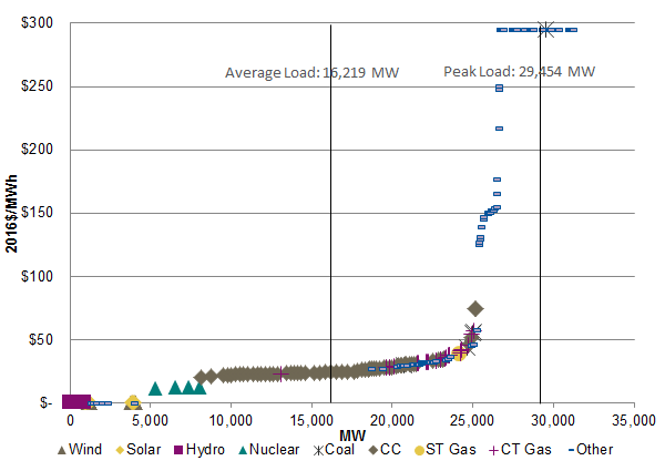
| Year | CC | CT Gas | ST Gas | Hydro | Nuclear | Other Renewable | Solar | Wind |
|---|---|---|---|---|---|---|---|---|
| 2017 | 688 | 0 | 0 | 0 | 0 | 0 | 1,205 | 338 |
| 2018 | 751 | 285 | 0 | 0 | 0 | 0 | 103 | 143 |
| Year | ST Gas | CT Gas | CT Other | Nuclear | ST Coal | ST Other |
|---|---|---|---|---|---|---|
| 2017 | 0 | 0 | 0 | 0 | 1,099 | 435 |
| 2018 | 0 | 0 | 0 | 0 | 0 | 0 |
| Month | Gas | Coal | Oil |
|---|---|---|---|
| January | $8.64 | $2.90 | $10.93 |
| February | $8.61 | $2.90 | $10.89 |
| March | $5.33 | $2.90 | $10.83 |
| April | $3.05 | $2.90 | $10.82 |
| May | $2.65 | $2.90 | $10.89 |
| June | $2.71 | $2.90 | $10.90 |
| July | $2.77 | $2.90 | $10.85 |
| August | $2.74 | $2.90 | $10.83 |
| September | $2.48 | $2.90 | $10.82 |
| October | $2.50 | $2.90 | $10.80 |
| November | $3.36 | $2.90 | $10.86 |
| December | $6.26 | $2.90 | $10.95 |
Appendix C. NYISO modelling assumptions
The following figures and tables summarise Navigant’s key assumptions for the abovementioned jurisdiction.
Figure 17. NYISO 2018 Supply Stack
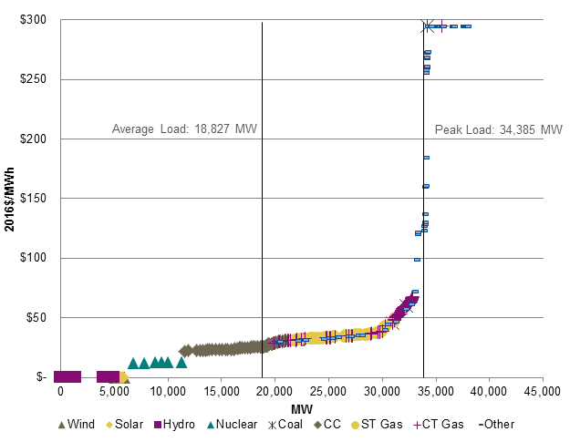
| Year | CC | CT Gas | ST Gas | Hydro | Nuclear | Other Renewable | Solar | Wind |
|---|---|---|---|---|---|---|---|---|
| 2017 | 0 | 0 | 0 | 0 | 0 | 0 | 878 | 78 |
| 2018 | 706 | 0 | 0 | 0 | 0 | 21 | 387 | 105 |
Figure 19. NYISO Capacity Retirements
No retirements in 2017 or expected in 2018.
| Month | Gas | Coal | Oil |
|---|---|---|---|
| January | $7.76 | $2.87 | $9.39 |
| February | $7.74 | $2.87 | $9.32 |
| March | $4.23 | $2.87 | $9.24 |
| April | $2.90 | $2.87 | $9.45 |
| May | $2.67 | $2.87 | $9.59 |
| June | $2.74 | $2.87 | $9.54 |
| July | $2.74 | $2.87 | $9.37 |
| August | $2.74 | $2.87 | $9.39 |
| September | $2.65 | $2.87 | $9.39 |
| October | $2.73 | $2.87 | $9.34 |
| November | $3.11 | $2.87 | $9.28 |
| December | $4.60 | $2.87 | $9.38 |
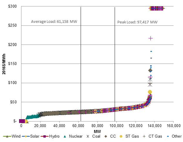
Appendix D. PJM modelling assumptions
The following figures and tables summarise Navigant’s key assumptions for the abovementioned jurisdiction.
Figure 20. PJM 2018 Supply Stack
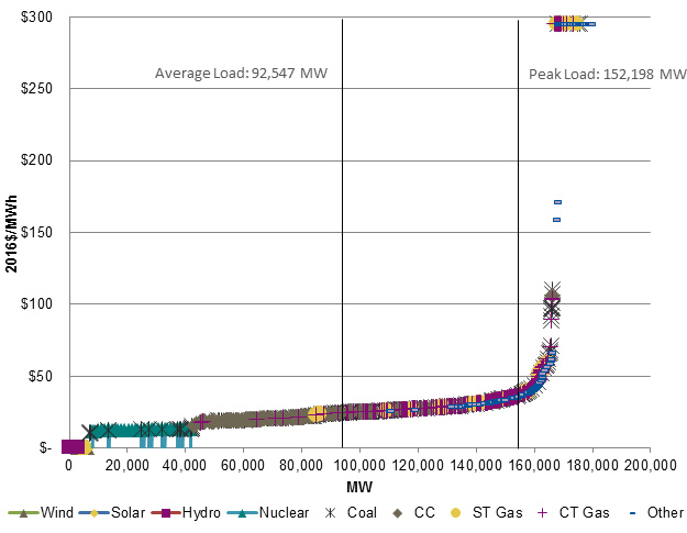
| Year | CC | CT Gas | ST Gas | Hydro | Nuclear | Other Renewable | Solar | Wind |
|---|---|---|---|---|---|---|---|---|
| 2017 | 5,069 | 21 | 543 | 0 | 0 | 0 | 3,839 | 572 |
| 2018 | 4,516 | 0 | 148 | 0 | 0 | 160 | 1,145 | 255 |
| Year | ST Gas | CT Gas | CT Other | Nuclear | ST Coal | ST Other |
|---|---|---|---|---|---|---|
| 2017 | 0 | 0 | 0 | 0 | 3,444 | 143 |
| 2018 | 34 | 0 | 0 | 0 | 2,819 | 0 |
| Month | Gas | Coal | Oil |
|---|---|---|---|
| January | $3.12 | $2.44 | $10.57 |
| February | $3.13 | $2.44 | $10.55 |
| March | $3.07 | $2.44 | $10.50 |
| April | $2.78 | $2.44 | $10.59 |
| May | $2.73 | $2.44 | $10.72 |
| June | $2.72 | $2.44 | $10.76 |
| July | $2.73 | $2.44 | $10.70 |
| August | $2.69 | $2.44 | $10.69 |
| September | $2.64 | $2.44 | $10.68 |
| October | $2.68 | $2.44 | $10.67 |
| November | $2.73 | $2.44 | $10.63 |
| December | $2.84 | $2.44 | $10.67 |
Appendix E. MISO modelling assumptions
The following figures and tables summarise Navigant’s key assumptions for the abovementioned jurisdiction.
Figure 23. MISO 2018 Supply Stack
| Year | CC | CT Gas | ST Gas | Hydro | Nuclear | Other Renewable | Solar | Wind |
|---|---|---|---|---|---|---|---|---|
| 2017 | 1,482 | 291 | 418 | 9 | 0 | 0 | 1,918 | 945 |
| 2018 | 0 | 39 | 117 | 18 | 0 | 0 | 101 | 250 |
| Year | ST Gas | CT Gas | CT Other | Nuclear | ST Coal | ST Other |
|---|---|---|---|---|---|---|
| 2017 | 0 | 0 | 138 | 0 | 1,621 | 0 |
| 2018 | 201 | 0 | 0 | 750 | 199 | 0 |
| Month | Gas | Coal | Oil |
|---|---|---|---|
| January | $3.15 | $2.31 | $8.97 |
| February | $3.14 | $2.31 | $8.92 |
| March | $3.08 | $2.31 | $8.84 |
| April | $2.70 | $2.31 | $8.90 |
| May | $2.59 | $2.31 | $9.00 |
| June | $2.58 | $2.31 | $9.02 |
| July | $2.57 | $2.31 | $8.93 |
| August | $2.57 | $2.31 | $8.90 |
| September | $2.54 | $2.31 | $8.87 |
| October | $2.54 | $2.31 | $8.84 |
| November | $2.71 | $2.31 | $8.78 |
| December | $2.83 | $2.31 | $8.81 |
Appendix F. Comparison of 2017 and 2018 default emission factors
This section compares the 2017 and 2018 default emission factors and discusses the key drivers of change for each region.
F.1 ISO-NE
ISO-NE has seen an overall decrease in emission factors which is driven by:
- Retirement of the last large coal plant, and
- Increases in renewable generation and CC gas capacity.
| Time-Of-Use | 2017 | 2018 | Change |
|---|---|---|---|
| Peak | 0.480 | 0.414 | -14% |
| Off Peak | 0.344 | 0.297 | -14% |
F.2 NYISO
Similar to ISO-NE, NYISO has also seen an overall decrease in emission factors which is driven by increases in renewable generation and CC gas capacity.
| Time-Of-Use | 2017 | 2018 | Change |
|---|---|---|---|
| Peak | 0.510 | 0.434 | -15% |
| Off Peak | 0.352 | 0.311 | -12% |
F.3 PJM
In 2017, PJM had coal on the margin during the off-peak and a mix of coal and gas on the margin during the peak which resulted in a higher emission factor for the off-peak period. In 2018, the lower gas prices make it more economical to dispatch gas plants during the off-peak periods which combined with significant increases in CC gas capacity and renewable generation as well as some coal retirements result in:
- a mix of coal and gas (weighted to gas) being on the margin during the off-peak period lowering the emission factor, and
- a mix of coal and gas (weighted more to coal) on the margin during the peak increasing the emission factor.
| Time-Of-Use | 2017 | 2018 | Change |
|---|---|---|---|
| Peak | 0.605 | 0.754 | +25% |
| Off Peak | 0.812 | 0.607 | -25% |
F.4 MISO
In 2017, similar to PJM, MISO had coal on the margin during the off-peak and a mix of coal and gas on the margin during the peak which resulted in a higher emission factor for the off-peak period. Increased renewable generation coupled with lower gas prices in 2018 make it more economical to dispatch gas plants during the off-peak periods which results in more gas being on the margin in the off peak thereby resulting in a lower off-peak emission factor.
| Time-Of-Use | 2017 | 2018 | Change |
|---|---|---|---|
| Peak | 0.789 | 0.768 | -3% |
| Off Peak | 0.965 | 0.730 | -24% |
Footnotes
- footnote[1] Back to paragraph Appendix F compares the 2017 and 2018 default emission factors.
- footnote[2] Back to paragraph Forward looking assumptions for each region can be found in the appendix.
- footnote[3] Back to paragraph Fuel costs can be found in the appendices which contain the modelling assumptions for each region.
- footnote[4] Back to paragraph California Air Resources Board – Chapter 3: What does my company need to do to comply with the cap and trade regulation? Section 3.8 Additional Requirements for Electric Utilities
- footnote[5] Back to paragraph Regulation respecting mandatory reporting of certain emissions of contaminants into the atmosphere.
- footnote[6] Back to paragraph Quebec updated its default emission factors in 2017.
- footnote[7] Back to paragraph Appendix F compares the 2017 and 2018 Default Emission Factors.
- footnote[8] Back to paragraph Navigant expects gas prices to decline from 2017 to 2018. For example, at the Henry Hub Navigant expects a decline of 15%.
- footnote[9] Back to paragraph The 'Other' category is mostly oil peaking units but encompasses landfill, biomass, waste heat, Steam Turbine / Combustion Turbine / Internal Combustion oil units, and Combustion Turbine kerosene units.
- footnote[10] Back to paragraph The 'Other' category is mostly oil peaking units but encompasses landfill, biomass, waste heat, Steam Turbine / Combustion Turbine / Internal Combustion oil units, and Combustion Turbine kerosene units.
- footnote[11] Back to paragraph The 'Other' category is mostly oil peaking units but encompasses landfill, biomass, waste heat, Steam Turbine / Combustion Turbine / Internal Combustion oil units, and Combustion Turbine kerosene units.
- footnote[12] Back to paragraph The 'Other' category is mostly oil peaking units but encompasses landfill, biomass, waste heat, Steam Turbine / Combustion Turbine / Internal Combustion oil units, and Combustion Turbine kerosene units.