Water quality of 15 streams in agricultural watersheds of Southwestern Ontario 2004-2009
The Nutrient Management Programme, led by the Environmental Monitoring and Reporting Branch of the Ontario Ministry of the Environment, is an on-going study of the impacts of agricultural activities on stream water quality in Southwestern Ontario. In this document, we report on data collected from 2004-2009 as part of this programme.
Prepared by: Ontario Ministry of the Environment
Environmental Monitoring and Reporting Branch
Last Revision Date: August 2012
Cette publication hautement spécialisée n’est disponible qu’en anglais en vertu du règlement 441/97, qui en exempte l’application de la Loi sur les services en français. Pour obtenir de l’aide en français, veuillez communiquer avec le ministère de l’Environnement au 416 327-1851.
For more information:
Ministry of the Environment Public Information Centre
Email: picemail.moe@ontario.ca
Website: Ministry of the Environment and Climate Change
© Queen’s Printer for Ontario, 2012
PIBS 8613e
Executive Summary
Southwestern Ontario is a region of intense crop and livestock production. The impacts of these agricultural activities on stream water quality is a concern for the health of the streams flowing through these regions, as well as downstream receiving waters, including large rivers with drinking water intakes and the Great Lakes. The Nutrient Management Programme, led by the Environmental Monitoring and Reporting Branch of the Ontario Ministry of the Environment, is an on-going study of the impacts of agricultural activities on stream water quality in Southwestern Ontario. In this document, we report on data collected from 2004-2009 as part of this programme.
- We examined 15 streams in Southwestern Ontario that were in agriculturally-dominated watersheds and received no point-source anthropogenic inputs. This region of Ontario is among the most intensive regions in terms of livestock and manure production in Canada.
- Streams were sampled for water quality and discharge. While several water quality parameters were measured, we report here on nitrite plus nitrate (NO2+NO3), total phosphorus (TP), suspended solids (SS), and Escherichia coli (E. coli) concentrations in the study streams and the loads of these substances delivered by them.
- Median TP concentrations of samples collected at the streams ranged from 18 µg P L-1 (Silver and Salem Creeks) to 156 µg P L-1 (Nissouri Creek), with median TP concentrations exceeding the Provincial Water Quality Objective (PWQO) for TP of 30 µg P L-1 in 9 of the 15 study streams.
- Median NO3- concentrations of samples collected at the streams ranged from 2.8 mg-1 (Blyth Brook) to 8.1 mg-1 (Nineteen Creek), with median NO3- concentrations exceeding the Canadian Council of Ministers of the Environment (CCME) guideline for nitrate of 2.93 mg -1 in 14 of the 15 study streams.
- Median E. coli concentrations of samples collected at the streams ranged from 93 CFU 100 mL-1 (Nineteen Creek) to 1400 CFU 100 mL-1 (Nissouri Creek).
- Estimates of stream loads of all the water quality parameters reported here varied considerably among streams. Mean annual NO2+NO3 loading varied approximately 3-fold, TP and SS almost 10-fold, and E. coli almost 100-fold among the study streams.
- We compared stream loading estimates from the present work to a study of agricultural streams in the same region approximately 30 years ago (PLUARG). Several estimates of loading between the two periods were similar, while in several other cases, our loading estimates were appreciably higher than those found by the PLUARG study.
- There were marked seasonal patterns in nutrient concentrations and loads, with a majority of annual loads of TP, NO2+NO3, and SS delivered in winter and early spring with low loading of these substances during summer.
- The seasonal pattern of E. coli loading and concentration differed from nutrients (TP and NO2+NO3) and SS. E. coli loads were highest during autumn while their concentrations were at their peak in midsummer to early autumn (July to October).
- The per cent of total stream flow occurring as base flow varied considerably among streams, ranging from 46% (Little Ausable River) to 72% (Muskrat Creek).
- Relationships between census-level land use data and water quality suggest that cattle and poultry density in the study watersheds were positively related to TP and E. coli concentrations.
- Using the preliminary data that were available, we found no relationship between the number of Nutrient Management Plans implemented in a watershed and any of the measured stream water quality indicators.
- Further work (underway) on stream invertebrates and diatoms will provide more information on the biotic health of these streams.
- Fine-scale land-use data, currently being obtained from OMAFRA, will likely improve our ability to relate land use to stream water quality.
Acknowledgements
The current Nutrient Management team consists of Pradeep Goel, Chris Jones, Georgina Kaltenecker, Mohamed Mohamed, and Dave Supper at the Environmental Monitoring and Reporting Branch of the Ontario Ministry of the Environment.
Georgina Kaltenecker conducted spatial analyses, including watershed delineation, analyses of geology, land use, spatial census data, producing geographical maps, and assisted with the development of the sampling design.
Aaron Todd, Pradeep Goel, and Saloni Clerk designed the programme, including site selection and sampling design as well as conducting field sampling and data analyses.
Beth Gilbert and Lisai Shen collected samples, maintained sampling equipment, and conducted previous analyses.
Dave Supper designed, constructed and maintained key sampling equipment as well as assisted with sampling.
Rory Gallaugher provided assistance with sample retrieval and compilation of precipitation and discharge data, as well as assistance with the calculation of stream loads and base flow separations.
Carline Rocks and Shenaz Sunderani assisted with data retrieval and discussion regarding sample quality assurance.
Deborah Conrod provided discussion and guidance on project management.
Duncan Boyd provided discussion, guidance, and critique of an earlier draft of this report.
Keith Somers and William Taylor provided advice with statistical analyses.
Krista Chomicki, Mike Christie, Pradeep Goel, Vasily Rogojin, Janis Thomas, and Aaron Todd provided valuable discussion and critique on earlier drafts of this report.
The Upper Thames Region, Long Point Region, and Maitland Valley Conservation Authorities collected water samples, conducted regular measurements of stream discharge, and provided advice on site suitability and sampling logistics. Several summer students have assisted with stream sampling during the programme.
Scott Abernethy and Hugh Geurts (South West Region, Ministry of the Environment), Mari Veliz (Ausable Bayfield Conservation Authority), Clara Tucker (Source Water Protection Branch, Ministry of the Environment) and several reviewers from the Ontario Ministry of Agriculture, Food and Rural Affairs provided valuable comments on an earlier draft of this report.
Introduction
Improvements in agricultural production have been, in part, due to the application of nutrients to crops to improve their yield (Stewart et al. 2005). Nutrients can be applied to crops in the form of synthetic fertilisers, the use of which increased dramatically in the ‘green revolution’ from the 1940s to the 1970s (Vitousek et al. 1997). Agriculture source material, mostly in the form of manure, is another major source of nutrients used in some farming operations. Manure contains, to varying degrees, the same nutrients contained in synthetic fertilisers, though the chemical forms of these nutrients can vary compared to synthetic fertilisers. Additionally, manure contains organic carbon and various other substances, such as microbes and insoluble particulates.
The use of these nutrients has greatly increased crop production and our ability to produce adequate food to sustain human populations. Some nutrients, as well as other agriculture source materials, however, are lost from farms to surrounding streams (Carpenter et al. 1998). In the same way that nutrients are added to crops to increase their growth, they can they can increase the growth of algae and aquatic plants in receiving waters. This increased algae and plant growth can have deleterious effects on streams and lakes receiving nutrient effluent from agricultural inputs. Their presence can be a nuisance, causing aesthetic impairment of waters and can result in the production of odour-causing growths. Effects that are far more serious can also occur. While less common, excessive nutrients can result in the production of toxic algae. Overgrowth of algae and aquatic plants can also affect the environment of the receiving waters (e.g. reduction in O2 concentrations) which can dramatically alter the types of organisms capable of surviving in those environments. The alteration of the aquatic environment can also affect the environmental services provided by the receiving waters (e.g. rates of nutrient and organic matter processing).
Two important nutrients associated with agricultural operations that can potentially enter streams are phosphorus and nitrogen. For freshwaters, phosphorus is the primary nutrient that results in eutrophication (Smith 2003). Thus, excess phosphorus is the most likely nutrient to lead to the overgrowth of algae and plants and the potential cascade of effects that can result from it. Streams receiving excess phosphorus might show such visible symptoms of eutrophication. Additionally, some of the phosphorus entering these streams will be transported downstream, potentially resulting in eutrophication of the larger streams or lakes receiving their inputs. Phosphorus arriving to streams is often sediment-bound with much of this sediment-bound fraction unavailable, to varying degrees, to aquatic organisms (e.g. Logan, 1982). A typically smaller fraction of phosphorus arriving to streams from agricultural inputs is in a dissolved, and typically more labile, form. The balance between dissolved and sediment-bound phosphorus is dynamic, with the forms exchanging between each other. It is exceptionally difficult to determine the biologically available fraction of phosphorus from the refractory fractions. Thus, total phosphorus (TP), which includes virtually all forms of phosphorus, is often used as a measure of phosphorus in aquatic systems.
Agriculturally sourced nitrogen can enter streams in a variety of forms. The most oxidised forms, NO2+NO3 are especially important to consider. Many stream organisms are sensitive to high concentrations of NO2+NO3. At higher concentrations, NO2+NO3are also a concern for human health as they interfere with oxygen metabolism (Sandstedt 1990). While secondary in its importance in the overgrowth of algae and aquatic plants when compared to phosphorus, NO2+NO3can result in shifts in the relative abundance of algae, potentially increasing the growth of undesirable forms.
Aside from nutrients, other agriculturally produced materials, such as insoluble particulates, can be significant to receiving waters. When moving with the stream flow, these insoluble particles are known as suspended solids (SS) and contribute to turbidity in stream water. These can be lost from the landscape and into streams through natural erosion. Human activities, including agriculture, have the potential to dramatically increase erosion and the subsequent SS they produce. Activities such as the alteration of stream banks and the cultivation of land adjacent to streams can result in increased sediment runoff. Additionally, alterations to channel morphology can cause increased downstream transport of stream sediment. As described above, a large portion of stream phosphorus is typically sediment-bound, so increases in stream SS can be coupled with increased stream phosphorus concentration.
Faecally-derived microbes can also be lost to waterways through run-off following land application of manure or from pasturing of livestock. The most commonly measured indicator of faecal contamination is the bacterium Escherichia coli (E. coli). Common inhabitants of the digestive system of warm-blooded animals, most strains of E. coli do not cause disease in humans. Since they are easily cultured and identified, however, E. coli are used as an indicator of recent faecal contamination of water and therefore the possible presence of faecal pathogens (Anon 2009).
Agriculture source material can enter stream water through different pathways. Soluble materials (e.g. NO2+NO3) travel primarily by infiltration through the soil, arriving to the stream through interflow, agricultural drains, or ground water. Conversely, insoluble materials (e.g. SS) arrive to streams primarily through overland flow. Many substances can have fractions that behave as if soluble with other fractions behaving as if insoluble (e.g. E. coli and TP). An important determinant of the relative balance of overland versus infiltration inputs to streams is the soil porosity. An understanding of relative soil porosity, as well as other features that can modify transport pathways in watersheds (e.g. agricultural drainage) can lend insight into the potential for various watersheds to transport agriculture source material to streams.
When assessing the potential environmental consequences of the nutrients, SS, and microbes described above, it is important to consider the possible impacts to the streams that are directly receiving these inputs as well as water bodies such as rivers and lakes that indirectly receive these inputs. Firstly, processing of materials is different in small streams, larger streams, and in lakes. For example, it has been found that small streams are much more important in the removal of nitrate than are larger streams (Alexander, Smith, & Schwarz 2000). The impacts on receiving waters can also be very different from the impacts that occur in small, agricultural streams. An example of this is the effect of phosphorus inputs. In some small streams, elevated phosphorus might not result in excessive algal or aquatic plant growth, if light or the substratum is unsuitable. However, when this phosphorus is delivered to larger streams and lakes, it can result in such overgrowth of algae or attached plants because of different environmental conditions (e.g. more light and/or slower moving water; Moran & Woods 2009). Another reason to consider potential impacts on receiving waters separately from those of the agricultural streams receiving these inputs is that our use of these waters is often quite different. While small agricultural streams are not typically used for drinking water or recreation, their water is often ultimately delivered to rivers or lakes that are used for these purposes. When considering in-stream effects, the concentration of a substance is typically the unit of interest. In contrast, the potential impacts on downstream receiving waters are often best understood by considering the mass of material, or load, delivered by the stream.
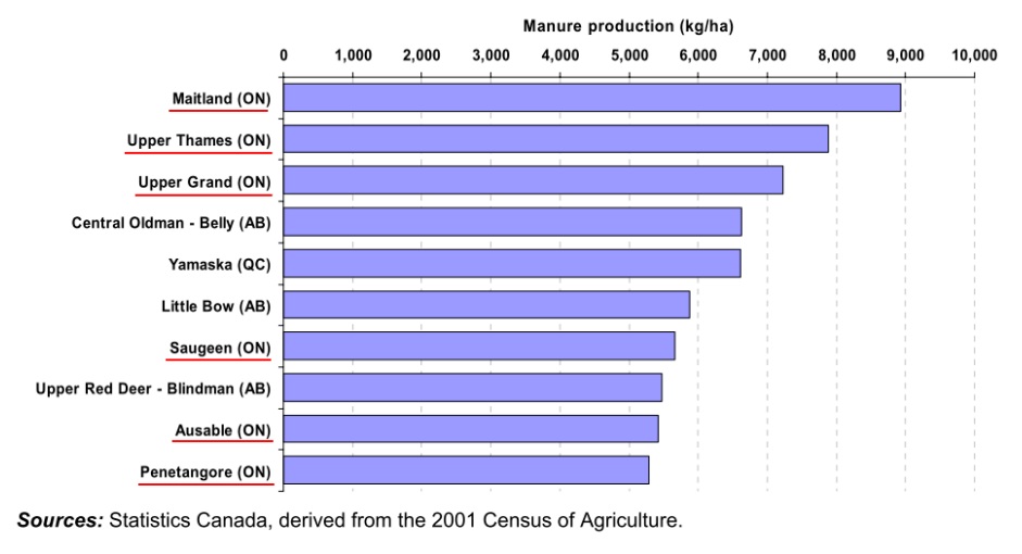
The extent to which streams are impacted by agricultural activities is related, in part, to the intensity of agriculture in the region. Southwestern Ontario is a region of intense agriculture, with high livestock densities and manure production. A study on manure production by Hoffman & Beaulieu (2006) found that several watersheds in Southwestern Ontario were among the highest producers of manure in Canada (Figure 1). Their work showed that these watersheds ranked similarly high in their production of nitrogen and phosphorus.
Figure 1: The ten sub-sub-drainage basins with the highest manure production in Canada (2001 Census of Agriculture). Watersheds in Southwestern Ontario are underlined in red. Figure modified from Hoffman and Beaulieu (2006).
While some of the types of farming activities that are practiced in Southwestern Ontario have changed in recent years, this region has been one of high agricultural and livestock production for several decades. In the late 1970s and early 1980s, it was intensively studied by the Pollution from Land Use Activities Reference Group (PLUARG). One of the main goals of the PLUARG project was to quantify inputs to the Laurentian Great Lakes from land use activities (Ongley 1978). A component of this work was to determine the contributions from agricultural activity and assess their potential impacts on the Great Lakes (Anon 1983). The PLUARG project studied several small watersheds in Southwestern Ontario and used the relationship between loading rates of nutrients and sediments with land use to develop a model to estimate inputs of these materials from all agricultural streams in the Great Lakes Basin (Coote & DeHaan 1978). The authors of the PLUARG work concluded that agricultural activity was a significant contributor of nutrients to the Great Lakes and had the potential to exacerbate eutrophication of those lakes. Their work also proposed several mitigation strategies to reduce runoff from agriculture (Anon 1983).
While the intensity of agricultural land use is an important factor in its environmental impact, the types of land uses employed on farms are also important in determining the degree of environmental impact. Practices that can reduce the loss of nutrients and other materials, known as “best management practices” (BMPs), have been developed. In Ontario, the Nutrient Management Act (NMA; O.Reg. 267/03) was created to provide consistent province-wide rules to regulate farm activities related to nutrient management (Environmental Commissioner of Ontario 2004).
As stated in the NMA, its purpose is, “to provide for the management of materials containing nutrients in ways that will enhance protection of the natural environment and provide a sustainable future for agricultural operations and rural development.”. The original regulation came into force on September 30th, 2003 and has been amended since (O.Reg. 511/05, Environmental Commissioner of Ontario 2004). A few of the requirements of the NMA pertain to all types of farms that apply agricultural or non-agricultural source materials. However, the main focus of regulation are livestock operations (Environmental Commissioner of Ontario 2006).
The PLUARG work described above was the last time agriculturally-dominated streams and their watersheds were systematically studied in Southwestern Ontario in this way. In this new work, we examined the water quality of several small, agriculturally-dominated streams situated in a Southwestern Ontario. Our specific goals were to:
- Measure concentrations of nutrients (TP, NO2+NO3), E. coli, and SS in these streams from 2004 to 2009. Combining these with discharge measurements, we calculated loads of these substances delivered by a subset of these streams to receiving waters.
- Observe seasonal trends in loads and concentrations, discussing their implications.
- Compare water quality observed in the study streams to the larger watersheds in which they are contained.
- Consider the potential in-stream consequences of TP, NO2+NO3, SS, and E. coli by examining stream concentrations as well as consider potential impacts to receiving waters by examining loading of these substances to the study streams.
- Compare the concentration and load estimates we generated to the pre-anthropogenically impacted estimates for these measures of water quality as well as to loading estimates generated during the PLUARG study of the same region.
- Use census-scale land use information to assess whether any broad-scale relationships between land use and stream water quality were evident.
Methods
Study watersheds
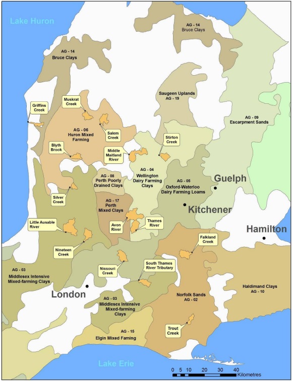
The locations of the study watersheds are shown in Figure 2 (detailed maps of each watershed are shown in the Appendix). Most of the study watersheds are part of the sub-sub drainage areas identified by Hoffman & Beaulieu (2006) as being among the top 10 manure-producing regions in Canada (Figure 1, Table 1). The study watersheds were also selected to meet several additional criteria:
- land use in each watershed was predominately agricultural and each watershed contained several farm operations;
- there were no urban or industrial point sources; and
- there was a variety of soil types and geology among watersheds.
Additionally, the outlet of each watershed, where sampling was done, had to be easily and publicly accessible. These requirements constrained the range of watershed areas used in this study from 11 km-2 (Silver Creek) to 58 km-2 (Little Ausable Creek), with an average watershed area of 26 km-2. Agricultural use comprised an average of 85% of the land area in the watersheds, ranging from 64% at Blyth Brook to 96% at Silver Creek. Forest ranged from 3% (Silver Creek) to 35% (Trout Creek) of watershed area. Wetland comprised a very small portion of the watersheds. The Blyth Brook watershed had the highest proportionate area of wetland at 3.5% of the total area. Urban development was generally absent from the study watersheds. The Trout Creek watershed, however, contains the hamlet of Pine Grove (population approx. 200) while the Falkland River watershed contains the hamlet of Princeton (population approx. 500). Neither of these communities discharge waste through a point source to the study streams.
As alluded to in the Introduction, our study watersheds also fell into zones identified by the PLUARG. Several agricultural streams were studied intensively in the PLUARG work and many regions with agriculture as the dominant land use were identified. The PLUARG regions were delimited based on areas with similar soils, geology, and agricultural land use, with the aim of generating generalised relationships between land use and stream water quality in each region (Chesters et al. 1978). Two of our study watersheds (Nissouri Creek and the Little Ausable River) were also examined in the PLUARG work.
Figure 2: Watersheds (orange) used in the present study. Labels indicate the watershed outlet, where samples were collected. Corresponding PLUARG regions (e.g. “AG-04”) and soil type in which each study watershed is located are indicated. Detailed maps of study watersheds are shown in the Appendix.
| Watershed | PWQMN ID | Lat. |
Long. |
Area (km-2) | Major watershed | Ultimate drainage | PLUARG region | % Agriculture |
% Forest |
% Wetland |
% NMP |
|---|---|---|---|---|---|---|---|---|---|---|---|
| Avon | 040013103 | 43.38 | -80.94 | 51.7 | Thames | St. Clair | 4 | 88 | 10 | 0.1 | 1 |
| Blyth | 080056044 | 43.73 | -81.38 | 17.5 | Maitland | Huron | 6 | 64 | 30 | 3.5 | 2 |
| Falkland | 160184123 | 43.18 | -80.43 | 29.8 | Grand | Erie | 2 | 85 | 10 | 0.6 | 7 |
| Griffins | 080056049 | 43.92 | -81.71 | 12.8 | Penetangore | Huron | 14 | 95 | 4.4 | 0.0 | 38 |
| Little Ausable | 080022014 | 43.29 | -81.41 | 57.9 | Ausable | Huron | 3 | 95 | 4.5 | 0.0 | 7 |
| Middle Maitland | 080056043 | 43.74 | -80.92 | 46.3 | Maitland | Huron | 4 | 87 | 10 | 0.3 | 7 |
| Muskrat | 080123060 | 43.98 | -81.27 | 20.7 | Saugeen | Huron | 6 | 73 | 22 | 0.6 | 16 |
| Nineteen | 040013100 | 43.24 | -81.27 | 26.4 | Thames | St. Clair | 3 | 95 | 5.5 | 0.0 | 9 |
| Nissouri | 040013034 | 43.13 | -80.96 | 30.9 | Thames | St. Clair | 5 | 86 | 12 | 1.0 | 21 |
| Salem | 080056050 | 43.91 | -81.15 | 26.3 | Maitland | Huron | 6 | 77 | 20 | 0.9 | 14 |
| Silver | 080040011 | 43.55 | -81.39 | 10.6 | Bayfield | Huron | 3 | 96 | 3.1 | 0 | 28 |
| South Thames | 040013101 | 43.02 | -80.85 | 22.1 | Thames | St. Clair | 3 | 95 | 5.0 | 0.2 | 38 |
| Stirton | 160184118 | 43.73 | -80.69 | 20.0 | Grand | Erie | 4 | 96 | 4.0 | 0 | 0 |
| Thames | 040013102 | 43.31 | -80.87 | 29.8 | Thames | St. Clair | 4 | 88 | 0.5 | 0.5 | 15 |
| Trout | 160124014 | 42.78 | -80.48 | 14.3 | Long Point | Erie | 2 | 64 | 35 | 0.5 | 0 |
Soil Porosity
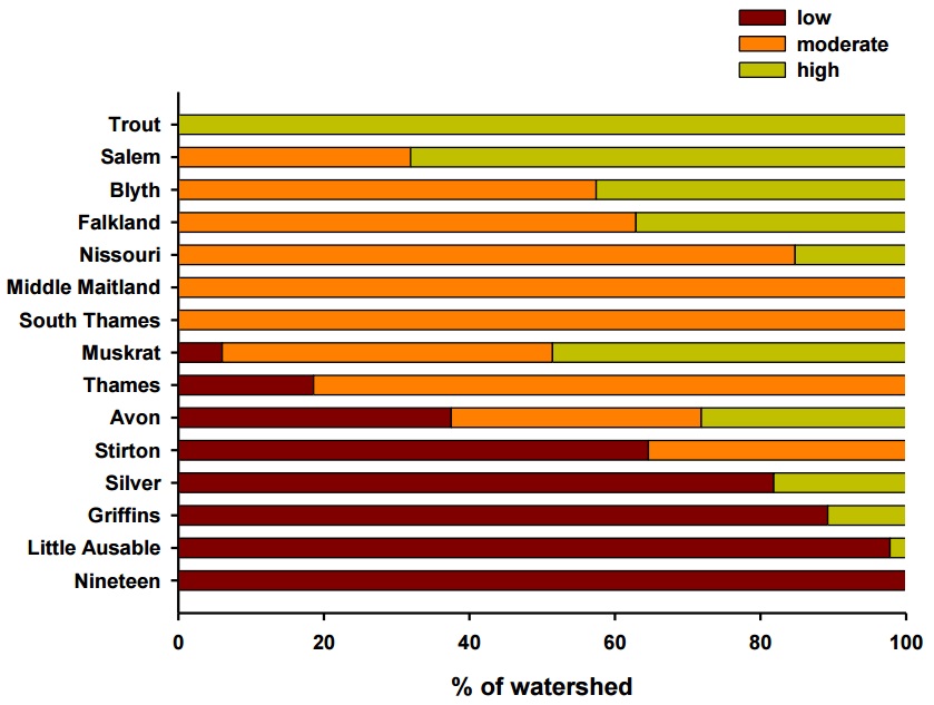
There is a broad range of soil porosity in the study watersheds (Figure 3) with no clear north-south or east-west gradients in soil porosities. The Trout and Falkland Creek watersheds, located in Norfolk Sands, have entirely high-porous and a mix of highly- and moderately-porous soils, respectively. The watersheds of The South Thames Tributary, The Little Ausable River, Nineteen Creek, and Silver Creek, all located in Middlesex Intensive Mixed-farming clays, range from having entirely moderately-porous soils (South Thames) to having entirely low- porosity soils (Nineteen Creek). Nissouri Creek, in Oxford-Waterloo Dairy Farming Loams is predominated by moderately-porous soils. While the Thames River, Stirton Creek, and the Middle Maitland River watersheds are all located in Wellington Dairy Farming Clays, they range in porosity from having entirely moderate-porosity soils (Middle Maitland) to having predominantly low- porosity soils (Stirton). The Blyth Brook, Muskrat Creek, and Salem Creek watersheds, all in the Huron Mixed Farming region, generally have a mix of moderate and high-porosity soils, though the Muskrat Creek watershed has a small proportion of low-porosity soil. The Griffin’s Creek watershed, located in the Bruce Clays, is dominated by low-porosity soil.
Figure 3: Proportion of low, moderate, and high porosity soils in the study watersheds. Data from Ministry of Mines and Northern Development Quaternary Geology 1:1,000,000 scale.
Stream sampling
Sampling for water quality and discharge was done at the watershed outlet 12 to 15 times per year at each sampling site. Sampling was not done on fixed intervals. Rather, it was done in an effort to capture a mixture of base flow as well as high flow events (e.g. spring melt and storm events). An effort was made to capture as many high-flow events as possible, as these are important in the models that we used to calculate stream loads (see “Stream Loads” section below). Sampling for water quality samples followed the methods used for PWQMN sampling (Todd 2006). Samples were transported to and analysed by Laboratory Services Branch (LaSB) at the Ministry of the Environment. While a wide variety of water quality parameters were measured, this report focuses on NO2+NO3, NO3-, TP, turbidity/suspended solids, and E. coli. Concentrations for NO3-, NO2+NO3, and TP are reported as the concentration of the element of interest.
During water quality sampling, field measurements for dissolved oxygen, pH, and water temperature were also collected with a YSI 600 QS multiparameter sonde. Additionally, stream velocity was measured at a minimum of 10 subsections across a stream transect (close to the site where water quality samples were collected) using a Marsh McBirney flow meter. Stream stage readings, from a staff gauge deployed at each site, were also recorded during sample collection. Continuous measurements of stream level were recorded with Leveloggers (Solinst), deployed at each stream. Measurements of stream velocity were used to generate estimates of stream discharge (see “Continuous discharge” below).
At one of the study streams (Nissouri Creek), we have collected more detailed stream water quality information. We measure stream turbidity at near-continuous frequency and conduct automated sampling of water quality during storm events at this station. While not presented in the this report, this more intensive sampling strategy will allow for more accurate assessment of stream loading and will serve as the basis for modelling of stream loading at this watershed.
Precipitation data
We obtained precipitation data from Environment Canada stations that were as close as possible to the study watersheds. In addition to their proximity to the study watersheds, we used only data from weather stations with reasonably complete data records (i.e. fewer than approximately 5 missing days of data in any month). In total, we used data from 5 stations spread across the study region (Table 2). Precipitation data from the years that the PLUARG loading estimates were done were also compiled. While data were not available for all the same Environment Canada stations as we used, we compiled data from six stations representing roughly the same geographical area as the present work.
| Watershed | Closest weather station | Climate ID | Distance to sampling site (km) |
|---|---|---|---|
| Avon | London CS | 6144478 | 42 |
| Blyth | Kincardine | 6124127 | 53 |
| Falkland | Waterloo | 6144239 | 33 |
| Griffins | Kincardine | 6124127 | 29 |
| Little Ausable | London CS | 6144478 | 35 |
| Middle Maitland | Elora RCS | 6142286 | 41 |
| Muskrat | Kincardine | 6124127 | 35 |
| Nineteen | London CS | 6144478 | 25 |
| Nissouri | London CS | 6144478 | 18 |
| Salem | Kincardine | 6124127 | 47 |
| Silver | Thedford | 612HKLR | 55 |
| South Thames. | London CS | 6144478 | 23 |
| Stirton | Elora RCS | 6142286 | 22 |
| Thames | London CS | 6144478 | 37 |
| Trout | Delhi CS | 6131983 | 12 |
Agricultural land use in the watersheds
Using census data, we estimated manure production, and their N and P equivalents, in each watershed. Along with other farm operation information, the available agricultural census data (from Statistics Canada, 2001) provided information on the type and number of livestock. We calculated manure production from cattle, pigs, and poultry, which are the three major livestock operation types in our study watersheds. Since information on the application of manure was not available, we assumed that manure produced in a watershed was applied in the same watershed. Livestock of other types generally form a minor part of the total livestock production in these watersheds, and are not detailed in the Statistics Canada information. In the census data, pigs, poultry, and cattle are further divided into subcategories. These subcategories match closely with those of Hofmann and Beaulieu (2006) who provide estimates of manure, N, and P production by each of these subcategories. Subcategories used from Hofmann and Beaulieu (2006) are shown in Table 3.
| Livestock Type | Average mass (kg indiv-1) |
Manure (kg indiv-1 y-1) |
N (kg indiv-1 y-1) |
P (kg indiv-1 y-1) |
|---|---|---|---|---|
| Cattle: | ||||
| Beef cows (including bulls) | 635 | 13,444 | 78.8 | 21.3 |
| Calves | 204 | 4,321 | 25.3 | 6.9 |
| Heifers | 421 | 8,904 | 52.2 | 14.1 |
| Dairy cows | 612 | 22,706 | 122.0 | 26.8 |
| Steers | 454 | 9 603 | 56.3 | 15.2 |
| Pigs: | ||||
| Boars | 159 | 1,358 | 9.9 | 3.3 |
| Grower and finishing pigs | 61 | 1,287 | 8.5 | 3.2 |
| Nursing and weaner pigs | 11 | 613 | 3.5 | 1.4 |
| Sows and gilts | 125 | 1 358 | 9.6 | 3.1 |
| Poultry: | ||||
| Broilers, roasters, Cornish hens | 0.9 | 28 | 0.36 | 0.09 |
| Laying hens | 1.8 | 42 | 0.55 | 0.19 |
| Pullets | 0.9 | 28 | 0.36 | 0.09 |
| Other (including turkeys) | 6.8 | 117 | 1.54 | 0.57 |
The census data were available at the dissemination scale, which aggregates data from several farm units into larger areas. These dissemination areas (DAs) did not correspond with the study watersheds, however. Each of the study watersheds was generally composed of portions of several DAs. A geographical information system (GIS) was used to determine the proportion of each DA that was contained within a watershed. These proportions were then used to assign the number of livestock of each type within the study watersheds from each DA, which was done by summing the proportioned data from each DA that fell within a watershed’s boundaries. A key assumption in this method was that crops and livestock were evenly dispersed within each DA, such that the proportion of the DA captured by the watershed also represented the proportion of a particular crop or livestock category in the watershed.
A related data issue was that, when a DA contained a small enough number of livestock operations of a given type (cattle, pigs, and poultry) such that an individual operation could be identified, Statistics Canada suppressed information about those operations in an effort to protect privacy. In most cases of suppressed data, total livestock in a category (cattle, poultry, and pigs) were available and subcategory data were suppressed. In these cases, we assumed total livestock in a category were distributed among the subcategories based on the number of farms within that subcategory. Less commonly, the total livestock in a category were also suppressed. In these cases, we calculated the average number of livestock for each of the other DAs in the watershed that had data, and then applied this average per farm value for the farm or farms with suppressed data.
Continuous discharge
Stream velocities were measured by wading (see Stream Sampling above) and were converted to discharge by the method described by Rantz (1982). These were used with the staff gauge readings to generate a stage-discharge relationship at each sampling site. Continuous level data provided by the Leveloggers deployed at each stream would allow, in principle, the calculation of a continuous record of stream discharge at each site. Generating reliable stage-discharge relationships, however, proved to be problematic for a variety of reasons. These included the Leveloggers shifting position in the stream, from movement either during high stream flow or from intentional displacement by other stream users, as well as poor or unstable stage-discharge relationships at some sites. Additionally, it was difficult to capture the high flows needed to generate a stage-discharge relationship that would be applicable at all flows.
While it was not possible to calculate stream discharge at the nutrient monitoring sites using the stage-discharge relationships, at many of the sampling sites, we were able to generate an empirical relationship between wading discharge measured at the sampling site and discharge at a downstream Environment Canada gauge (Hydat). Watersheds, and the corresponding relationships between the measured wading discharge and the downstream Hydat station for which this approach was possible, are shown in Table 4. At one of the sampling sites (Avon), a Hydat station is located at the Nutrient Management site, so we were able to use these discharge data directly.
As discharge among the streams varied considerably, when considering the monthly pattern in discharge among streams, we expressed discharge as the per cent of annual discharge in each month. When comparing annual patterns in discharge, we standardised discharge among the streams using z-scores, which represent each observation as their standard deviation from the mean.
Stream loads
Stream load is defined as the mass of a substance (either suspended or soluble) carried by the stream. For those streams where we were able to calculate daily discharge, it was generally possible to generate estimates of stream load. While there are several types of approaches to modelling stream loads, we found that for the small, fast responding streams in this study, combined with the type of data we had available for the study streams (infrequent water quality data combined with frequent discharge data), regression-based approaches appeared to provide the best estimates of stream loading.
We generated load estimates using the Microsoft Windows-based software package, Loadrunner. Loadrunner acts as a user-interface for the Fortran-based program Loadest, which is produced by the United States Geological Survey. Provided with intermittent water quality and daily discharge measures, Loadest develops estimates of stream load using 9 models of varying complexity that relate the measured concentrations to stream discharge. Based on the Akaike Information Criterion (AIC; a statistical estimate of model fit), Loadest recommended the appropriate model with which to estimate load, as well as providing other statistical measures to assess the validity of the model fit. To generate accurate estimates of stream load, it is important to have concentration data at a variety of stream discharge rates. This is especially true for high flows, during which the relationship between flow and concentration can differ greatly from that of lower flows. To achieve this, we combined the data from the several years for which we had concentration and discharge data, generating a single model to determine stream load for all years. This approach increased the range of flow and concentration data to generate the model, allowing for more valid model fits. An assumption required in this approach is that the relationship between concentration and discharge did not vary from year to year.
Load estimate outputs were evaluated for normality and a lack of trend in residuals. The adjusted maximum likelihood estimation (AMLE), a parametric method, was applied to estimate loads when these conditions were met. In the case of NO2+NO3 loads at the Middle Maitland River, we found a trend in residuals so we used a non-parametric method (least absolute deviation; LAD) to estimate loads of NO2+NO3 at this stream.
| Watershed | Relationship to Hydat gauge | r2 |
|---|---|---|
| Blyth Brook | 0.27x0.76 | 0.88 |
| Little Ausable River | 0.30x + 0.02 | 0.95 |
| Middle Maitland River | 0.49x | 0.91 |
| Muskrat | 0.16x0.97 | 0.94 |
| Nineteen | 0.16x | 0.96 |
| Nissouri | 0.09x | 0.94 |
| Silver | 0.64x + 0.02 | 0.95 |
| South Thames | 0.02x1.3 | 0.84 |
To compare stream loads from the various watersheds, we standardised them by expressing them as unit-area loads. For year-to-year comparisons among streams, we standardised the unit-area loadings for each water quality measure against the mean load for each stream using a z-score. This approach allowed a year-to-year comparison among streams, even though the unit-area loadings varied widely among streams.
Inferred stream concentrations
The grab samples we collected were sparse in number and the sampling regime emphasised high-flow events (see “Stream Sampling” section above). Thus, the grab samples do not provide an estimate of average or typical conditions in the streams. However, the loading estimates we calculated also provided corollary concentration data. These concentrations are time-weighted mean concentrations (TWMC), representing the average concentration for a given time period. TWMC serve as a way to estimate what the stream concentrations were on a daily basis, without requiring the collection of a prohibitively large number of field samples. While loading data provide an estimate of the total mass of substances delivered to receiving waters, TWMC in the streams provide an estimate of the average concentrations experienced by organisms in a stream. In this way, TWMC provide a useful estimate of the potential ecological impact to a stream, while loading estimates provide an estimate more relevant to potential impacts on receiving water bodies.
There are some important caveats in the interpretation of TWMC data. Firstly, because the estimate of TWMC is based on loading, the assumptions and considerations involved in the loading estimates must also be applied to TWMC estimates. As mentioned above, TWMC represent the average concentration in a given period. Since our discharge data were daily values, the minimum period we can estimate is a daily average. Because of this, and because these concentrations are inferred from loading, TWMC are not directly analogous to the instantaneous measure of concentration provided by a grab sample.
Base flow separation
Due to solubility differences, some materials (e.g. NO2+NO3) are more likely to travel through groundwater and subsurface flow (base flow) than via runoff and overland flow (quick flow). Differing proportions of base flow among streams could have implications for the relative importance of pathways by which nutrients could be transported. Additionally, the proportion of stream flow attributable to base flow might vary seasonally with variations in precipitation, recharge, and evapo-transpiration. For those streams for which we were able to infer continuous discharge (see “Continuous Discharge” above, we conducted hydrograph separation analyses to estimate the relative amount of flow that was provided by base flow versus the amount provided by quick flow. We performed hydrograph separations using a two-parameter recursive digital filter using the Web-based Hydrograph Analysis Tool (WHAT; Lim et al. 2005). There are several numerical methods for hydrograph separation available and it is known that these methods can produce different values for flow attributed to stream base flow (Eckhardt 2008). Thus, our base flow separations should be viewed as relative estimates of base flow among streams, rather than absolute measures, which typically require tracer experiments to establish (Sklash et al. 1978).
Comparison with PLUARG values
As mentioned, the study streams are located in regions used in the PLUARG studies and two streams, Nissouri Creek and the Little Ausable River, were used in both the present study and in the PLUARG work. We compared loading estimates for streams in the present study that were also in the streams of the PLUARG studies, as well as against the more generalised regional PLUARG loading estimates.
Comparisons of loading estimates between the PLUARG work and those of our study require some caution and should only be made for general comparison. While two of the PLUARG streams are the same as ours, the other streams are only in the same PLUARG region, and variability among streams within a PLUARG region is likely. The PLUARG study estimated nutrient and sediment loads using the Beale Ratio estimator, which could generate different estimates from the regression-based approach we use for our data. Perhaps more significantly, the PLUARG loading values were generated from a far more intensive sampling effort. We were unable in the present study to sample every high-flow event. These high-flow events are important in generating loading models and can result in modelled loads that are an underestimate (Runkel, Crawford, & Cohn 2004), especially for insoluble compounds (e.g. suspended sediment, and sediment-bound portions of E. coli and TP). Thus, our loading estimates for TP, E. coli, and SS are likely to be greater underestimates than for NO2+NO3. The PLUARG loading estimates were based on 2 years of data (1975 and 1976) while ours were based on 4 years of data. Since stream loadings can vary appreciably from year to year, this should also be taken into account when comparing loading values.
Statistical analyses
For summary statistics of water quality measures collected at the sampling sites, we generally used the non-parametric descriptors (median, nonparametric percentiles) of these values. This is because stream water quality data are typically highly variable, often non- normal in distribution, and prone to high- outliers. Use of the median and nonparametric percentiles will reduce bias from high outliers in the data.
We explored relationships in land use among watersheds with principal component analysis (PCA). PCA is a multivariate statistical technique that reduces the original variables (in our case, crop and livestock densities) to a smaller number of aggregate variables referred to as principal components (PCA), which explain most of the variance in the data (O’Rourke et al. 2005). We used a biplot to display the results of the PCA, in which the original land use variables (crop and livestock densities) are shown as vectors on the plot of the PC axes. The length and direction of these vectors is related to their relative influence on each PC axis. Additionally, the study watersheds are shown as points on the PC axes, with their relative positions suggesting their relationship to the PC axes as well as the vectors of the original variables. PCA is sensitive to the scaling of variables. Since our land use measures were in different units, we standardised them by conducting the PCA on the correlation matrix, rather than the covariance matrix of the data (Quinn and Keough 2002). Because multivariate techniques such as PCA can sometimes distort apparent relationships, we also explored the relationships between land use in the study watersheds with correlation analysis.
Similar to our approach to exploring the land use data, we used a related multivariate technique, redundancy analysis (RDA) to investigate the relationships between stream water quality and land use in the study watersheds. Like PCA, RDA generates aggregate variables, analogous to the PC axes (termed RD axes in RDA), to explain the variability in the data (Zuur et al. 2007). In RDA, however, variables are separated into environmental variables (in our case, land use) and response variables (in our case, water quality). The RDA attempts to explain the variability of the response variables in terms of the environmental variables. We displayed the results of the RDA as a triplot, in which environmental variables and response variables are shown as vectors. As with PCA, the direction and length of the environmental variables displays the extent to which they contribute to each of the RD axes. The length and direction of the response variables, in turn, displays their relationship to the environmental variables. Response and environmental variables in a similar direction imply a correlation between the two variables. Similar to PCA, the study watersheds displayed on the RDA triplot illustrate their relationship to the RD axes. As with the PCA, our variables were measured with differing units, so we conducted the RDA on the correlation matrix of the variables (Quinn and Keough 2002). Also similar to our analyses of the land use relationships, we examined the relationships between water quality and land use with correlation analysis between individual variables to evaluate potential relationships apparent in the RDA.
PCA and RDA analyses were performed using PAST (version 1.94b) and the Biplot add-in for Microsoft Excel (version 2.0). Correlation analyses were done using Sigmastat (version 3.5). Significant relationships in the correlation analyses were considered to be at p ≤ 0.05.
Results
Land use in the watersheds
Crop Types
Across all of the study watersheds, corn was the dominant crop type, with 25% coverage of the combined watershed area (Table 5). Grain, and forage and fodder each covered 12% and 11%, respectively, while soybean covered a slightly greater area at 16%. The per cent of area in grain production ranged from 5% to 31% of the total watershed area. The Stirton Creek watershed was the highest among the study watersheds in grain production, while the Nissouri Creek and South Thames River watersheds were the lowest. The Nissouri Creek and South Thames River watersheds had the highest corn production, with 40% corn coverage in their watersheds. Forage ranged from 2% (Trout Creek watershed) to 18% (Thames River and Middle Maitland River watersheds) of the watershed areas. Soybean area ranged from 8% (Salem) to 27% in the Silver Creek watershed, with the Little Ausable River, Griffins Creek, and Nineteen Creek watersheds each having a high proportion of land planted with soybean.
| Watershed | Grains | Corn | Forage and Fodder Crops | Soybean |
|---|---|---|---|---|
| Avon | 10 | 26 | 16 | 13 |
| Blyth | 8 | 17 | 6 | 15 |
| Falkland | 11 | 20 | 8 | 14 |
| Griffins | 14 | 28 | 14 | 21 |
| Little Ausable | 13 | 32 | 6 | 21 |
| Middle Maitland | 15 | 25 | 18 | 14 |
| Muskrat | 9 | 15 | 14 | 11 |
| Nineteen | 10 | 24 | 8 | 25 |
| Nissouri | 5 | 40 | 12 | 10 |
| Salem | 12 | 22 | 11 | 8 |
| Silver | 12 | 33 | 7 | 27 |
| South Thames | 7 | 40 | 16 | 20 |
| Stirton | 31 | 22 | 15 | 14 |
| Thames | 13 | 28 | 18 | 12 |
| Trout | 11 | 5 | 2 | 9 |
| Mean | 12 | 25 | 11 | 16 |
Livestock and manure production
Poultry density ranged from 91 indiv km-2 (Silver) to nearly 5000 indiv km-2 at the Stirton Creek watershed (Table 6). Cattle ranged from 6 indiv km-2 (Trout), with Stirton also having the highest cattle production at 116 indiv km-2 and Salem having similarly high numbers at 99 indiv km-2. Pig densities were the lowest at the Falkland and Griffins Creek watersheds (20 and 75 indiv km-2, respectively) and relatively high at several watersheds, including the watersheds of Nissouri Creek (354 indiv km-2), Silver Creek (379 indiv km-2), the South Thames Tributary (295 indiv km-2), and Stirton Creek (344 indiv km-2). Note that we were unable to determine pig density at Trout Creek. This was due to the small number of pig farms in the watershed, which resulted in data for all pig farms being suppressed by Statistics Canada in this watershed. As the total number of pig farms was low, however, it is unlikely that pig production was appreciable in the Trout Creek watershed.
| Watershed | poultry (indiv km-2) |
cattle (indiv km-2) |
pigs (indiv km-2) |
total manure (× 103 kg km-2 y-1) |
manure N (× 103 kg km-2 y-1) |
manure P (× 103 kg km-2 y-1) |
|---|---|---|---|---|---|---|
| Avon | 2427 | 51 | 349 | 790 | 5.3 | 1.6 |
| Blyth | 161 | 31 | 102 | 390 | 2.5 | 0.7 |
| Falkland | 339 | 25 | 20 | 220 | 1.4 | 0.4 |
| Griffins | 131 | 58 | 75 | 590 | 3.5 | 1.0 |
| Little Ausable | 1153 | 51 | 154 | 610 | 4.0 | 1.2 |
| Middle Maitland | 2932 | 74 | 128 | 840 | 5.6 | 1.5 |
| Muskrat | 1307 | 48 | 119 | 540 | 3.5 | 1.0 |
| Nineteen | 614 | 29 | 89 | 290 | 1.9 | 0.5 |
| Nissouri | 1844 | 57 | 354 | 870 | 5.6 | 1.7 |
| Salem | 348 | 99 | 182 | 1000 | 6.0 | 1.7 |
| Silver | 91 | 35 | 379 | 600 | 3.6 | 1.2 |
| South Thames | 722 | 60 | 295 | 770 | 4.7 | 1.4 |
| Stirton | 4939 | 116 | 344 | 1420 | 9.4 | 2.6 |
| Thames | 3181 | 64 | 244 | 820 | 5.7 | 1.7 |
| Trout | 1921 | 6 | 120 | 1.1 | 0.3 |
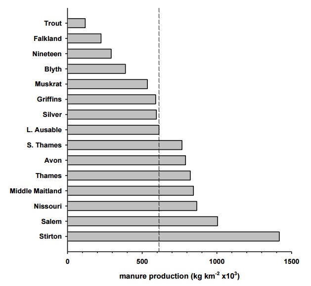
In line with their high livestock densities, the Stirton Creek and Salem Creek watersheds had the highest production of manure at 1420 × 103 kg km-2 y-1 and 1000 × 103 kg km-2 y-1, respectively (Figure 4). The lowest manure production was at the Trout Creek watershed (120 × 103 kg km-2 y-1) and the Falkland Creek watershed (220 × 103 kg km-2 y-1). In line with the high total manure production, the watersheds of Salem and Stirton Creeks also had the highest production of N generated from manure (6.0 and 9.4 × 10³ kg N km-2 y-1, respectively) while the lowest manure N was generated in the Trout Creek (1.1 × 10³ kg N km-2 y-1) and Falkland Creek watersheds (1.4 × 10³ kg N km-2 y-1). Manure P was also highest in the Stirton Creek watershed (2.6 × 10³ kg P km-2 y-1), though the Salem Creek, Nissouri Creek, and Thames River watersheds had the second-highest manure P production at 1.7 × 10³ kg P km-2 y-1 each. Note that because of the data suppression of pig production (see above), the total manure production in the Trout Creek watershed represents an underestimate.
Figure 4: Manure production in each study watershed arranged in order of increasing manure production. The dashed vertical line represents the median across streams.
Relationships among land use in the study watersheds
To provide some background description of agricultural land use, we examined the relationships among livestock densities and crops in the study watersheds. Generally, we found that livestock densities appeared to be positively related to each other (Table 7, Figure 5). Of these, however, only poultry density was significantly related to cattle density. The relationship between pig and cattle density appeared to be positive, though marginally non-significant, while the relationship between poultry and pig densities appeared to be positive, though non-significant. Poultry and grains appeared to be positively related, though this relationship was marginally non-significant. Pig density and corn were positively related among the study watersheds as was cattle and forage production. Soybean farming appeared to be negatively related to livestock production. It was significantly negatively related to both poultry and cattle density and suggested a negative relationship to pig density, though this relationship was found to be non-significant. Soybean density was unrelated to grain or corn density, while grain and corn densities were negatively related to each other.
| crop/livestock | pigs | cattle | poultry | soybean | forage | corn | |
|---|---|---|---|---|---|---|---|
| grains | p | −0.32 | 0.10 | 0.48 | 0.01 | −0.23 | −0.86 |
| grains | r | 0.24 | 0.73 | 0.07 | 0.97 | 0.41 | <0.001 |
| corn | p | 0.51 | 0.11 | −0.30 | −0.28 | 0.14 | |
| corn | r | 0.05 | 0.69 | 0.28 | 0.31 | 0.63 | |
| forage | p | 0.24 | 0.55 | 0.38 | −0.77 | ||
| forage | r | 0.40 | 0.03 | 0.17 | 0.001 | ||
| soybean | p | −0.43 | −0.74 | −0.55 | |||
| soybean | r | 0.11 | 0.002 | 0.03 | |||
| poultry | p | 0.35 | −0.52 | ||||
| poultry | r | 0.21 | 0.03 | ||||
| cattle | p | 0.48 | |||||
| cattle | r | 0.07 |
Figure 5: Principal components analysis showing relationships among land use in the study watersheds. Principal component (PC) axes are scaled to their relative contribution to the total variance explained (shown in brackets). Land use vectors are shown in blue while study watersheds are shown as grey points.
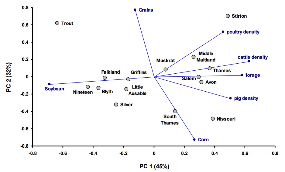
In the principal components analysis comparing land use in the watersheds (Figure 5), seventy-seven per cent of the variance among the land use characteristics was explained in the first two principal component (PC) axes. The first PC axis was not dominated by any single land use, with all variables except grains contributing appreciable loading to this axis. Variation in the second PC axis was dominated by grains, which loaded positively on this axis, against corn, which loaded negatively on the second PC axis. The watersheds of Nineteen, Blyth, and Falkland Creeks were especially high in soybean and low in cattle density and forage. Salem, Thames, Avon, and Middle Maitland showed the opposite pattern; high in cattle and forage, while low in soybean. Nissouri and South Thames were both high in corn and low in grain. The Trout Creek watershed showed a mix of grain and soybean, while it was low in corn and livestock. Note that the appearance of the Trout Creek watershed as an outlier on the PCA plot is likely due, in part, to the lack of pig density data that we have for that watershed.
Patterns in precipitation and relationship to stream discharge
The per cent of annual precipitation and discharge delivered in each month (from 2004 to 2009) are shown in Figure 6. Generally, while daily and weekly precipitation often varied considerably among the weather stations, when these were averaged on a monthly and annual basis, variability among the stations was relatively low. Thus, we averaged precipitation across all stations. The relatively high and variable precipitation in July was due largely to sporadic storms, especially at the Waterloo weather station.
The averaged pattern of precipitation and discharge are well summarised by a plot of monthly values. However, this also had the effect of obscuring the sporadic nature of flow events. In Figure 7, a plot of a single year at a single stream (the Little Ausable River in 2008) exemplifies a typical seasonal pattern in stream flow along with several variables that affect stream flow.
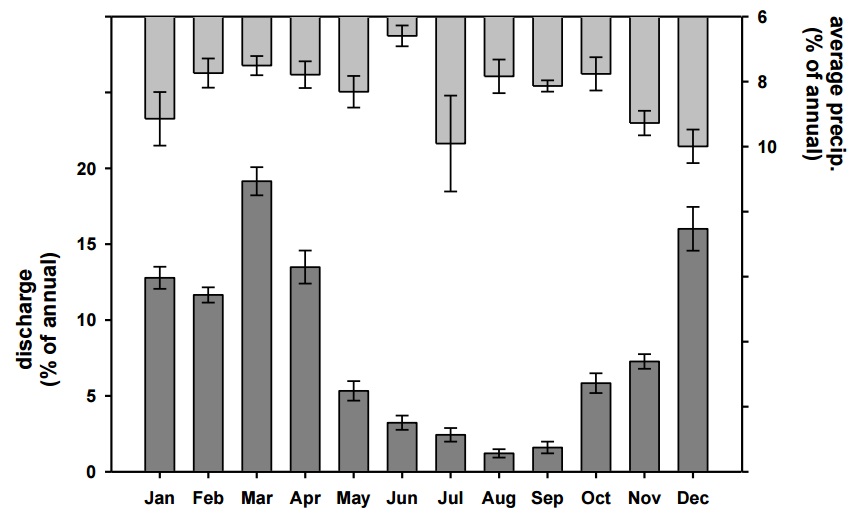
Figure 6: Per cent of discharge delivered each month for the streams having continuous discharge data (lower plot) and the per cent of annual precipitation delivered in each month across weather stations in the study region (upper plot). Error bars represent standard error of the mean and reflect variability among streams (discharge) and weather stations (precipitation).
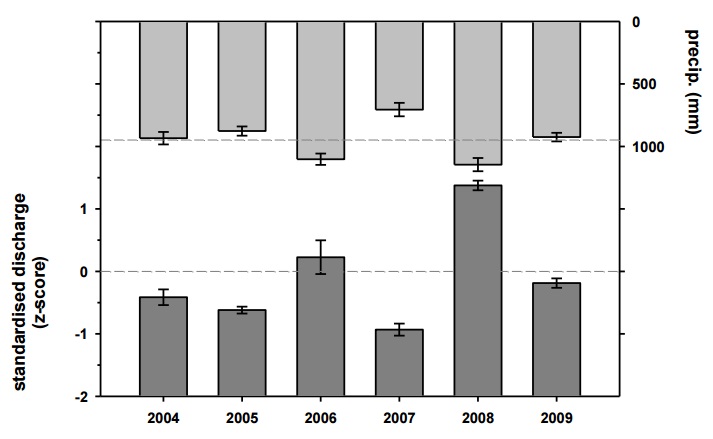
Summer discharge was typically very low, interspersed with short periods of moderately high flows from rain events. In autumn, short peaks in storm flows were overlaid on consistently high flows occurring from frequent rain events. While it was unusual for any of the study streams to dry at the sampling site, several of them would typically become stagnant, or nearly so, in midsummer. Winter (Dec. to Feb. inclusive) showed periods of below freezing temperatures and snow accumulation, interspersed by above-freezing temperatures that were often accompanied by rain, resulting in several high discharge events. While this pattern varied considerably among years (and among streams to a lesser extent), frequent winter rain/thaw events, with associated high discharge, were the norm for the study streams. Average annual precipitation across years was 948 mm, ranging from 705 mm in 2007 to 1146 mm in 2008 (Figure 8). Not surprisingly, annual precipitation and discharge followed similar patterns. Precipitation was above the 2004 to 2009 mean in 2006 and 2008 and below it in 2007. Similarly, in 2007, discharge was lower than the mean of the study years. However, discharge also appeared to be appreciably lower than the 2004 to 2009 mean in 2004 and 2005, even though precipitation was close to the mean for the years. Discharge was appreciably higher than the mean for the study period in 2008.
Figure 7: The Little Ausable River in 2008, showing discharge at the sampling station (separated into base- and quick flow), rainfall, air temperature, and snow on ground.
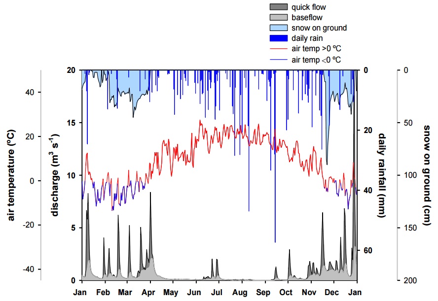
Figure 8: Annual precipitation and standardised annual discharge across the study streams. Dashed lines denote the mean discharge and mean precipitation among years. Error bars are standard error of the mean.
Stream discharge
For the nine streams for which continuous discharge was calculable, we noted a large variability in monthly discharge, typical of small, north temperate streams (Figure 6). August and September had the lowest mean monthly discharge, with 1.2 and 1.6% of annual discharge respectively, occurring in these months. In contrast, the highest mean monthly discharge occurred in March, with 19% of total discharge delivered in this month. Discharge was also high throughout the winter and early spring, with December, January, February, and April delivering 16, 13, 12, and 13% of annual discharge, respectively. All other months (May-July, October, and November) had monthly discharge ranging from 2.4 to 7.3% of annual discharge.
Patterns in base flow
For the subset of streams for which we were able to calculate continuous discharge, the range in the per cent of flow that was attributable to base flow among streams was considerable, ranging from 46% (Little Ausable River) to 72% (Muskrat Creek), based on data from 2006-2009 (Figure 9). The median per cent base flow among streams for those years was 54%. As anticipated, the proportion of flow attributable to base flow among streams followed a similar pattern as the proportion of porous soils among streams (Figure 3), with streams having more porous soils also showing relatively higher base flow compared to streams dominated by less porous soils.
The percentage of base flow also varied inter-annually (Figure 10). The years 2004-2006 were slightly below the average base flow among years while 2008, a year of high precipitation and discharge, was considerably below the average annual base flow. Conversely, 2007 was a relatively dry year and displayed higher than the average annual base flow.
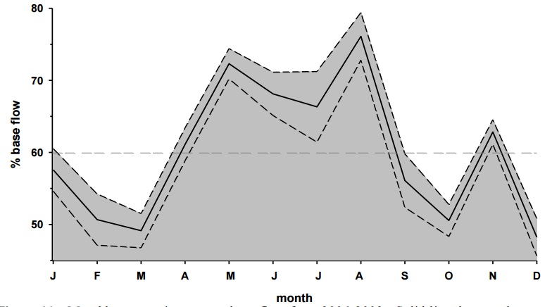
The monthly pattern in the percentage of base flow was that of low base flow contribution in winter, an increase in spring that remained high throughout summer, followed by a general decrease in late summer and autumn. An exception to this was November, which showed a slight resurgence in the proportion of base flow contribution (Figure 11).
Figure 9: Average per cent base flow in the study streams for which we could obtain continuous discharge, 2006-2009. Error bars are standard error of the mean, representing variation among years for each stream. The dashed vertical line represents the median base flow among streams.
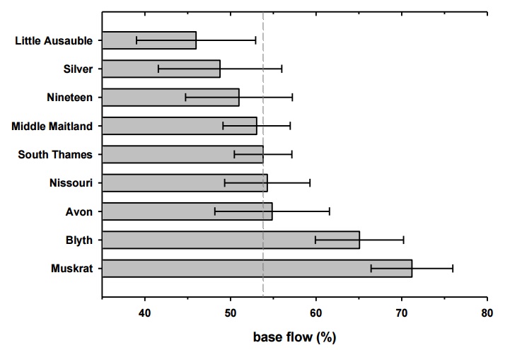
Figure 10: Annual base flow among streams, expressed as z-scores. Error bars are standard error of the mean, representing variability among streams. The dashed line represents the inter-annual average base flow. Note that for 2004 and 2005, data for only Blyth, Maitland, and Nissouri were available.
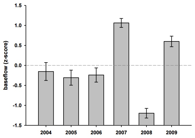
Figure 11: Monthly pattern in per cent base flow from 2006-2009. Solid line denotes the mean base flow among streams, while the dashed lines represent the upper and lower range, based on standard error of the mean among streams. The dashed horizontal line represents the mean annual base flow.
| measure | units | min | max | median | mean |
|---|---|---|---|---|---|
| TP | µg P L-1 | 2 | 129 | 33 | 70 |
| NO2+NO3 | mg N L-1 | below detection limit |
49.7 | 5.0 | 5.6 |
| NO3- | mg N L-1 | below detection limit |
49.5 | 5.0 | 5.6 |
| turbidity | FTU | 0.05 | 576 | 3.4 | 12.6 |
| E. coli | CFU 100 mL-1 | below detection limit |
1×10⁵ | 200 | 1425 |
Note that for E. coli, concentrations above or below method detection limits were set at the detection limit after determining that these incidences were low.
Measured water quality over the study period
Concentrations across streams and sampling dates
Concentrations of TP among streams and sampling dates ranged from 2 to 129 µg P L-1, with a grand median across all streams and sampling dates of 33 µg P L-1, slightly above the interim Provincial Water Quality Objective (PWQO) of 30 µg P L-1 (OMOEE 1994; Table 8). For NO2+NO3, the grand median concentration across all streams and sampling dates was 5.0 mg N L-1, ranging from below detection to 1×10⁵ CFU 100 mL-1, with a median across all streams and sampling dates of 200 CFU 100 mL-1.
Measured concentrations among streams
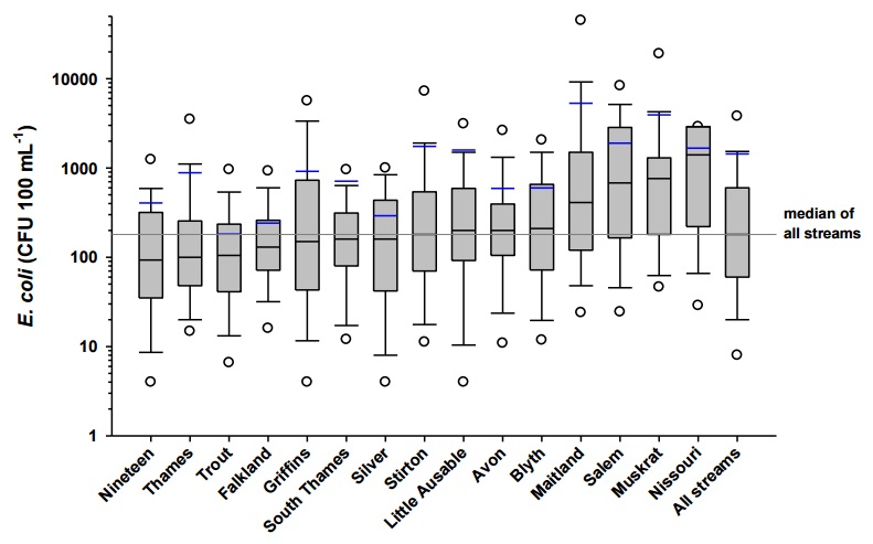
Median TP concentration among streams (for all sample dates; Figure 12) varied from 18 µg P L-1 (Silver and Salem Creeks) to 156 µg P L-1 (Nissouri Creek). Of the 15 study streams, 9 of the median TP concentrations exceeded the interim PWQO of 30 µg P L-1. Median NO2+NO3 concentrations (Figure 13) ranged from 2.8 mg N L-1 (Blyth Creek) to 8.1 mg N L-1 (Nineteen Creek). Median NO3- concentrations (Figure 14) ranged from 2.9 mg N L-1 (Trout Creek) to 7.9 mg N L-1 (Nineteen Creek). The median NO3- concentration of 14 of the 15 study streams exceeded the Canadian Council of Ministers of the Environment (CCME) guideline for protection of aquatic life. Median turbidity (Figure 15) ranged from 1.4 FTU (Silver and Salem Creeks) to 17.7 FTU (Nissouri Creek). Median E. coli concentrations among streams (Figure 16) varied from 93 CFU 100 mL-1 (Nineteen Creek) to 1400 CFU 100 mL-1 (Nissouri Creek).
Figure 12: TP concentrations sampled in the study streams, arranged in order of increasing median concentration. Dashed red line represents the interim PWQO for the prevention of eutrophication.
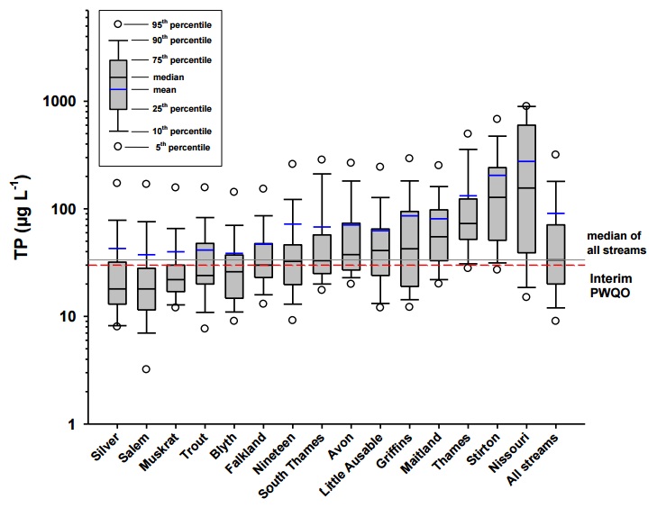
Figure 13: NO2+NO3 concentrations sampled in the study streams, arranged in order of increasing median concentration. Box definitions as in Figure 12.
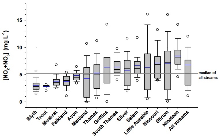
Figure 14: NO3- concentrations sampled in the study streams, arranged in order of increasing median concentration. Dashed red line represents the CCME guideline for the protection of aquatic life. Box definitions as in Figure 12.
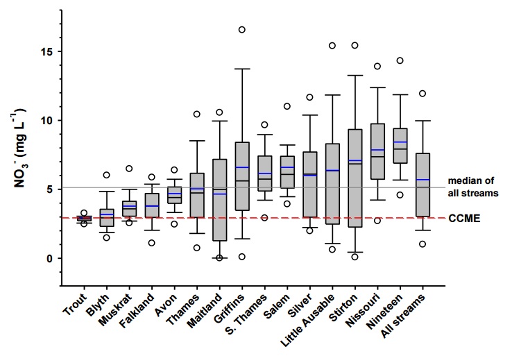
Figure 15: Turbidity sampled in the study streams, arranged in order of increasing median values. Box definitions as in Figure 12.
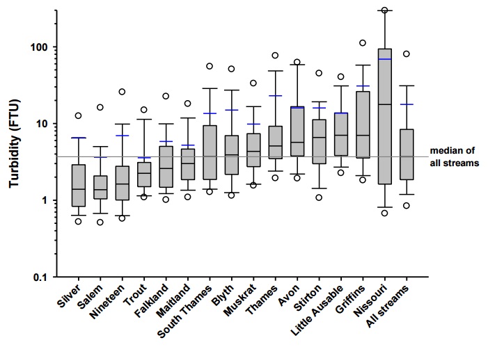
Figure 16: Summary of E. coli concentrations sampled in the study streams, arranged in order of increasing median concentrations. Box definitions as in Figure 12.
Nitrate and total phosphorus relative to other streams in the same major watershed
Data were compiled from the PWQMN stations for the major watersheds in which the streams of the present study were located to allow a comparison of concentrations of respective watershed. We noted especially high NO3- values relative to the median for the watershed, at Stirton Creek, which had a median NO3- concentration of 8 mg L-1 compared to the Grand River watershed, in which it is situated, at 2 mg L-1. Nineteen Creek and Nissouri Creek, with median NO - concentrations of 7 mg L-1 and 8 mg L-1, respectively, were considerably the same watershed. The majority of NO3- median concentrations from the present study were the same or slightly higher than the median of all streams monitored in their higher than the median for the watershed in which they are located (Upper Thames) of 4 mg L-1.
| Major watershed | Study stream | # of sites | NO3- (mg L-1) |
TP (µg L-1) |
|---|---|---|---|---|
| Ausable-Bayfield | 9 | 5 | 49 | |
| Little Ausable | 6 | 40 | ||
| Silver | 6 | 18 | ||
| Grand River | 36 | 2 | 42 | |
| Falkland | 3 | 32 | ||
| Stirton | 8 | 145 | ||
| Long Point | 9 | 3 | 59 | |
| Trout | 3 | 33 | ||
| Maitland Valley | 12 | 4 | 26 | |
| Blyth | 3 | 20 | ||
| Griffins | 6 | 41 | ||
| Middle Maitland | 5 | 55 | ||
| Salem | 6 | 20 | ||
| Saugeen Valley | 14 | 1 | 16 | |
| Muskrat | 3 | 22 | ||
| Upper Thames | 24 | 4 | 68 | |
| Avon | 4 | 41 | ||
| Nineteen | 7 | 32 | ||
| Nissouri | 8 | 44 | ||
| South Thames | 6 | 34 | ||
| Thames | 5 | 144 |
The situation appeared to be more variable for TP, with median concentrations at the study streams sometimes lower, similar to, or greater than, the median values of their respective larger watersheds. Silver Creek had a median TP concentration notably lower than the Ausable-Bayfield watershed, in which it is located (18 µg L-1 vs. 49µg L-1). The Avon River, Nineteen Creek, Nissouri Creek, and the South Thames River all had median TP concentrations appreciably lower than the median for the Upper Thames watershed as a whole (41, 32, 44, and 34 µg L-1 respectively, vs. 68 µg L-1 median TP for the Upper Thames). Conversely, some of the study streams had median TP concentrations far in excess of their respective watersheds. The median TP of Stirton Creek was far higher than the median for the Grand River as a whole (145 µg L-1 vs. 42 µg L-1). The Thames River median TP of 144 µg L-1 was also much higher than it was for the Upper Thames watershed (68 µg L-1).
Nutrient, suspended solid, and E. coli loading in the watersheds
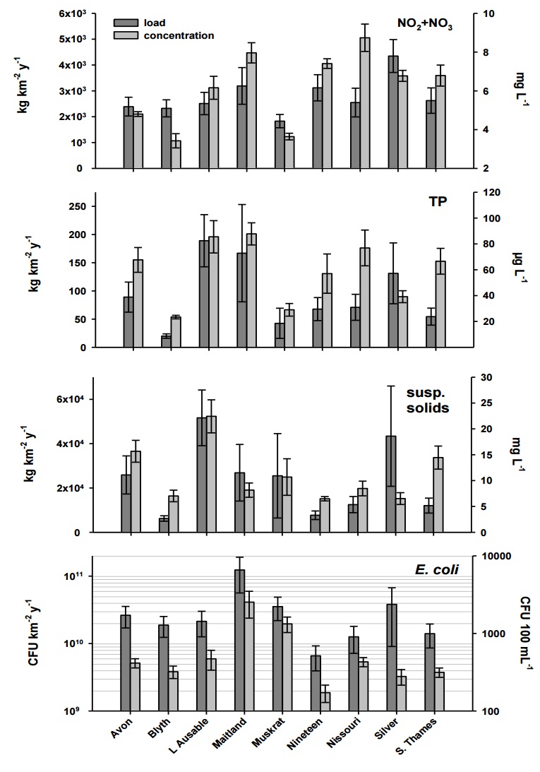
Among streams, we noted a greater than three-fold range in the unit area loading of N as NO2+NO3 (Figure 17). Average NO2+NO3 loading across streams and years was 2.8 × 10³ kg km-2 y-1. The highest loadings were from Silver Creek at 4.3 × 10³ kg km-2 y-1 while the lowest loading was from Muskrat Creek at 1.8 × 10³ kg km-2 y-1.
While the mass of TP delivered per unit area was much lower than that of NO2+NO3, the relative range in TP loading among watersheds was greater, spanning almost one order of magnitude. The highest average loading was at the Little Ausable River (189 kg km-2 y-1) with the second highest at the Middle Maitland River (167 kg km-2 y-1). The lowest TP loading was at Blyth Brook (20 kg km-2 y-1) and the average TP loading across streams and years was 92 kg km-2 y-1.
Suspended solids loading also spanned almost one order of magnitude among the study streams. As with TP, the Little Ausable River had the highest SS loading (5.2 × 10⁴ kg km-2 y-1) and Blyth Brook had the lowest (6.2 × 10³ kg km-2 y-1). Mean SS loading across years and streams was 2.4 × 10⁴ kg km-2 y-1.
E. coli loading spanned almost two orders of magnitude among streams. The Middle Maitland River had the highest E. coli loading at 1.2 × 10¹¹ CFU km-2 y-1 and Silver Creek was second highest at 3.8 × 10¹⁰ CFU km-2 y-1. We observed the lowest loadings of E. coli at Nineteen Creek of 6.6 × 10⁹ CFU km-2 y-1. Average loading of E. coli across streams and years was 3.3 × 10¹⁰ CFU km-2 y-1.
Figure 17: Mean unit-area loads and mean annual concentrations (as TWMC) at the study streams. Error bars are standard error of the mean.
Time-weighted mean concentrations among streams
Daily time weighted mean concentrations (TWMC) inferred from loadings generally followed the same pattern as loadings among streams, though this was not invariably the case (Figure 17). Generally, the range in TWMC was lower than that of stream loads.
TWMC of NO2+NO3 across streams and years was 6.2 mg L-1. Mean NO2+NO3 TWMC was highest at Nissouri Creek (8.7 mg L-1) while the lowest TWMC of NO2+NO3 were at Blyth Brook and Muskrat Creek (3.4 and 3.6 mg L-1, respectively).
While the range in TP loading was almost one order of magnitude, the range in TP TWMC among the watersheds was more constrained. The highest TWMC of TP were at the Little Ausable and Middle Maitland Rivers (both 90 µg L-1) and lowest at Blyth Brook (20 µg L-1), a range of 4.5-fold. Average TP TWMC across streams and years was 60 µg L-1.
As with TP, the range in SS TWMC was lower than that of loading, with the highest SS TWMC slightly less than 4 times that of the lowest TWMC. Suspended solid TWMC was highest at the Little Ausable River (22 mg L-1) and lowest at Nineteen Creek (6.5 mg L-1), with an average concentration of 11 mg L-1 across streams and years.
The range in E. coli TWMC, like TP and SS, was much smaller than that of loading. The highest E. coli concentrations were at the Middle Maitland River (2500 CFU 100 mL-1) and the lowest were at Nineteen Creek (170 CFU 100 mL-1), a range of just under 15-fold. The average E. coli TWMC across streams and years was 700 CFU 100 mL-1.
Exceedances of guidelines and objectives using TWMC
Using the inferred TWMC data, we predicted the number of days that the study streams (for which we could compute loads and TWMCs) were in exceedance of provincial guidelines. As mentioned previously, TWMCs (and therefore exceedances calculated using them) are not entirely analogous to grab samples (see Methods). Rather than representing a point- in-time sample, they reflect an estimate of the mean concentration on a daily basis. Thus, a single exceedance using TWMC values should be interpreted as the predicted mean concentration over an entire day in excess of the objective or guideline. An advantage of this approach is that it is not prone to potential bias introduced by a sampling scheme that is not very frequent and done on a regular basis throughout the year. Additionally, it provides information on chronic conditions in a stream. Daily fluctuations, however, are muted using TWMC approach, so the number of shorter- term exceedances would be underestimated using this method.
TP
The number of exceedances of the Provincial Water Quality Objective (PWQO) for TP varied widely among streams and, in some cases, among years within a stream (Table 10). Averaged across the study years, Blyth Brook had the fewest exceedances of the PWQO for TP, exceeding 30 µg L-1 27% of the time from 2004 to 2009. Nissouri Creek had the highest rate of exceedance, with TWMC of TP greater than 30 µg L-1 90% of the time across years. Some streams, such as the Middle Maitland River, varied little in their rate of exceedance from year to year. The range in this stream was a minimum of 80% of days in exceedance in 2007, to a maximum of 90% of days in exceedance in 2006. Nineteen Creek, conversely, ranged from a minimum of 52% of days in exceedance in 2009 to 100% of days in exceedance in 2006.
NO3-
For NO3- , there was a high rate of exceedance of the (CCME) guideline for the protection of aquatic life of 2.93 mg L-1 of NO3-N (Table 11). The Avon River, Nissouri Creek, and the South Thames Tributary exceeded the CCME for NO3- 100% of days for all years in which they were studied. The lowest rate of exceedance occurred at the Middle Maitland River, which exceeded the CCME guideline for NO3- on 59% of days from 2004 to 2009. Blyth Brook showed the greatest variation in NO3- exceedances among years, with only 25% of days in exceedance of the CCME guideline for NO3- in 2009, to 100% of days in exceedance in 2006 and 2007.
| Year | Avon | Blyth | Little Ausable | Muskrat | Nineteen | Nissouri | Silver | South Thames | Middle Maitland |
|---|---|---|---|---|---|---|---|---|---|
| 2004 | N/A | 59 | N/A | N/A | N/A | 91 | N/A | N/A | 81 |
| 2005 | N/A | 36 | N/A | N/A | N/A | 93 | 22 | 72 | 81 |
| 2006 | 83 | 24 | 75 | 21 | 100 | 99 | 41 | 89 | 90 |
| 2007 | 57 | 16 | 71 | 20 | 57 | 81 | 21 | 74 | 80 |
| 2008 | 99 | 16 | 81 | 45 | 66 | 93 | 47 | 90 | 85 |
| 2009 | 100 | 9 | 88 | 37 | 52 | 84 | 32 | 92 | 85 |
| mean | 85 | 27 | 79 | 31 | 69 | 90 | 33 | 83 | 84 |
| Year | Avon | Blyth | Little Ausable | Muskrat | Nineteen | Nissouri | Silver | South Thames | Middle Maitland |
|---|---|---|---|---|---|---|---|---|---|
| 2004 | N/A | 27 | N/A | N/A | N/A | 100 | N/A | N/A | 64 |
| 2005 | N/A | 86 | N/A | N/A | N/A | 100 | 93 | 100 | 54 |
| 2006 | 100 | 100 | 74 | 100 | 76 | 100 | 79 | 100 | 67 |
| 2007 | 100 | 100 | 59 | 83 | 100 | 100 | 79 | 100 | 31 |
| 2008 | 100 | 73 | 83 | 99 | 100 | 100 | 90 | 100 | 78 |
| 2009 | 100 | 25 | 66 | 80 | 100 | 100 | 85 | 100 | 61 |
| mean | 100 | 68 | 71 | 91 | 94 | 100 | 85 | 100 | 59 |
Year-to-year loadings in each of the study streams
All of the water quality measures followed a similar inter-annual pattern in loading and this pattern corresponded closely with that of annual discharge across the watersheds (Figure 8 and Figure 18). For example, 2007 had lower than average loadings of all water quality measures and also had lower than average discharge. In contrast, 2006 and 2009, years of higher than average discharge also demonstrated higher than average loadings. Note that, because the loading models we used are based on discharge and were developed assuming that the relationship between concentration and discharge were constant across the study years (see “Methods”), it is not surprising that the inter-annual pattern in loadings that we observed were driven largely by changes in discharge.
Figure 18: Annual load for each stream for each year (bars and left axes) and z-score of average load for each year (points and right axes).
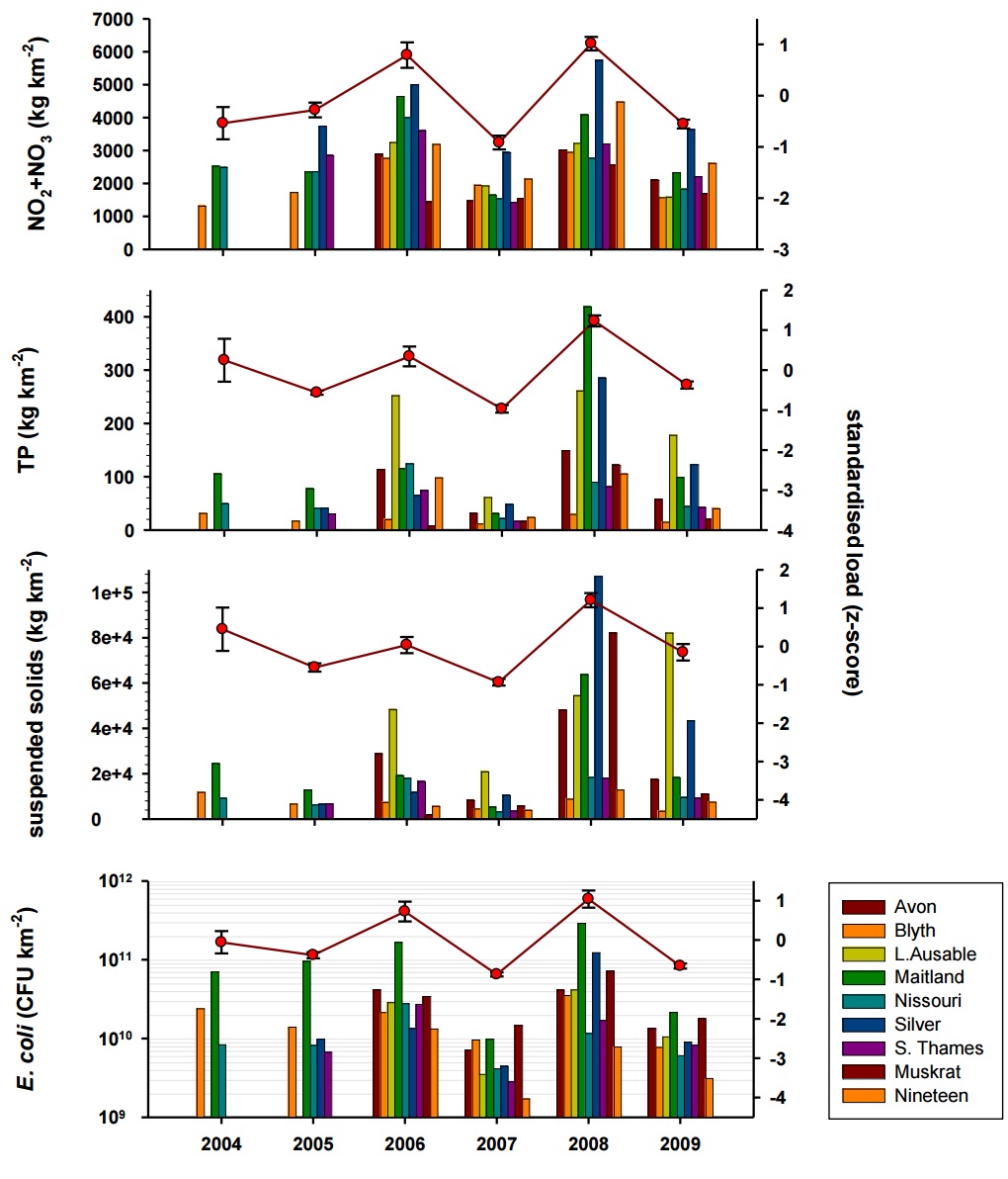
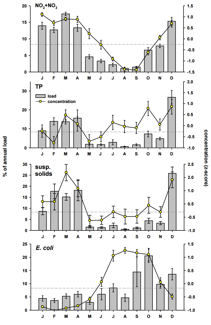
Figure 19: Per cent of annual load (bars, left axes) and monthly concentration expressed as z-scores (points, right axes) averaged across all of the study streams for which loadings were calculable. The dashed grey line represents the average annual load. Error bars are standard error of the mean, representing variability among streams.
Monthly and seasonal loads and concentrations
NO2+NO3
Both loading and concentration of NO2+NO3 followed similar intra-annual patterns (Figure 19). The lowest loads of NO2+NO3occurred in August and September, during which an average of approximately 2% of the annual load of NO2+NO3 was delivered to the streams. Loading of NO2+NO3 increased in October and November, and remained high from December to April. Each month from December to April contributed approximately 12 to 16% of the annual loading of NO2+NO3 to the study streams. On a seasonal basis, average NO2+NO3 loading was highest in winter, in which 42% of the NO2+NO3load was delivered to the study streams on average (Table 12). This was followed by spring, with 35% of the annual loading. The lowest NO2+NO3 loading occurred in summer, with 7% of the annual load delivered during the season. Similar to loadings, NO2+NO3 concentrations were the lowest during the summer months and high from December to April.
The monthly pattern in NO2+NO3 concentration was very similar to that of loading. As with loading, the lowest NO2+NO3 concentrations occurred in August and September, with an increase in October and November and steadily high NO2+NO3 concentrations throughout the winter until early spring. The concentration of NO2+NO3 declined after April, remaining low until October, corresponding to the decrease in loading.
TP
As with NO2+NO3 loads, average TP loading across the study streams was at its lowest in August, with approximately 1% of the average TP load delivered during that month. The highest TP loads were delivered in December, with 23% of the annual load delivered in the month, on average. TP loading remained relatively high from January to April, dropping off rapidly afterwards. The seasonal distribution of TP loading was similar to that of NO2+NO3. Half of the TP load was delivered during winter, and approximately one-third (31%) was delivered in spring. The remainder largely occurred in autumn (14%), with only 5% of the annual TP load delivered during summer.
| season | months | discharge | NO2+NO3 | TP | SS | E. coli |
|---|---|---|---|---|---|---|
| Winter | Dec-Feb | 41 | 42 | 50 | 52 | 22 |
| Spring | Mar-May | 38 | 35 | 31 | 35 | 14 |
| Summer | Jun-Aug | 7 | 7 | 5 | 4 | 19 |
| Autumn | Sept-Nov | 15 | 16 | 14 | 9 | 45 |
Unlike NO2+NO3, TP concentrations were not always temporally coherent with TP loading. While December was the highest in both concentration and loading, the relationship between loading and concentration, relative to their respective averages, varied from month to month in spring. For example, TP loading was above the monthly average in February, but concentrations were below average for the month. While TP loads remained low throughout summer, TP concentration remained close to the annual average TP concentration from approximately July to September. In October, TP concentrations were high, even though TP load during this month was relatively low.
Suspended solids
Suspended solids loading followed a similar pattern to that of TP, with relatively very low loading from May to September, a slight increase in October and November, the highest loading in December and sustained high loads through to April. Seasonally, only 4% and 9% of the suspended solid loading occurred in summer and autumn, respectively, while 52% occurred in winter and 35% occurred in spring.
Suspended solids concentration generally followed the same pattern as loading, though the highest SS concentrations occurred in March, rather than December, when loadings were at a maximum.
E. coli
E. coli loading followed a different pattern than that of the other three measures. The highest E. coli loadings occurred in October, during which approximately 21% of the annual E. coli load was delivered. However, the entire period from approximately September to December had relatively high loading of E. coli. In contrast, E. coli loading was relatively low in the period from January to August, with the lowest loading in May, during which approximately 3% of the annual load was delivered. Seasonally, the highest E. coli loads were delivered in autumn, with 45% of the E. coli loading occurring in that season. In the other seasons, loading was similar, at 22%, 14%, and 19% for winter, spring, and summer, respectively.
Figure 20: Per cent of annual load delivered in each month superimposed on per cent of base flow in each month.
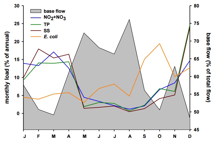
The pattern in the concentration of E. coli (as TWMC) was notably different from the monthly E. coli loading pattern. While loading from May to August did not greatly change, concentrations of E. coli increased from May to July and remained high from July to October. The autumn increase in loading was not reflected in E. coli concentration. Rather, E. coli concentration remained high for September and October, and then declined rapidly in November and December.
Base flow contribution to stream loads
For all of the water quality measures except E. coli, the per cent base flow appeared to show the opposite pattern to loading (Figure 20). The proportion of base flow was relatively high in summer and generally dropped in autumn and winter, while TP, NO2+NO3, and SS loading were low in summer and high in autumn and winter. The pattern in E. coli loading and base flow was less clear, as E. coli loadings remained low throughout winter but rose sharply from August to October, when the percentage of base flow was dropping.
Relationships among water quality measures
The only strong correlation among the water quality measures was between SS and TP (r=0.81, p=0.008; Figure 21), which showed an increase in TP with increasing SS. All other relationships were non-significant.
Figure 21: Correlation matrix between unit area loadings (kg km-2 y-1) of water quality variables.
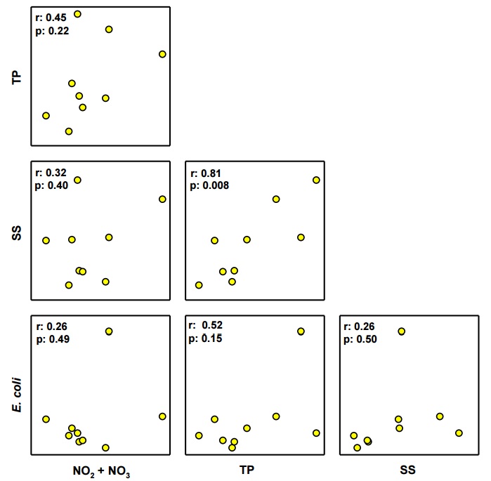
Relationships between land use and stream nutrient concentrations
We used redundancy analysis (RDA) to examine the relationships between land use (set as independent variables) and water quality variables (set as dependent variables; Figure 22). The first two axes of the RDA explained 77% of the variance between land use and water quality, with the first axis accounting for 46% of the total variance. Of the land use variables, most loaded in the same direction on the first axis. Notably, poultry density appeared to be closely related to TP concentration, while manure N, manure P, and cattle density appeared to be closely related to NO2+NO3 concentration and more weakly related to E. coli concentration. Both poultry density and cattle density appeared to be related to manure N and manure P produced in the watersheds. Interestingly, pig density only loaded weakly on the first axis, while grains and forage loaded only weakly on the first axis.
Figure 22: Redundancy analysis showing relationships between land use variables and time-weighted mean concentrations of water quality variables. Axes are scaled to represent the relative variance explained by each axis (shown in brackets). Blue lines represent environmental (land use) variables while red dashed lines represent response (water quality) variables (as concentrations). “BF” indicates the percentage of total discharge estimated to be base flow; “NMPs” represent the percentage of farms within a watershed captured under the Nutrient Management Act (2005, OMAFRA).
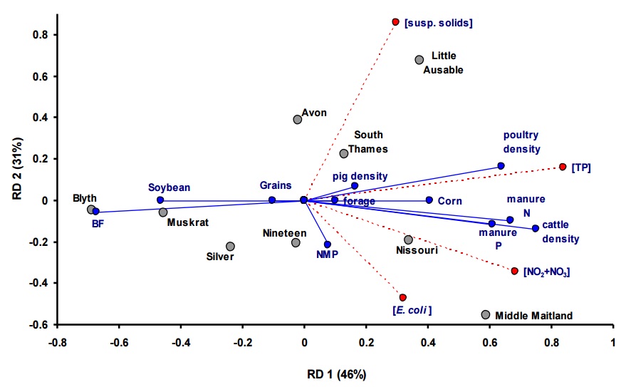
There were a few exceptions to the trend of the determining variables loading in the same direction. Firstly, soybean density and per cent base flow in the watersheds were negatively related to the other variables on the first axis. Second, the per cent nutrient management plans (NMPs) loaded weakly on the second axis, were roughly negatively related to SS concentration, and apparently unrelated to all of the other response and determining variables.
Of these streams for which we were able to calculate TWMC, the Middle Maitland River appeared at the extreme of high NO2+NO3 and E. coli concentration, while the Little Ausable River appeared at the extreme of high SS concentration. Blyth Brook, at the extreme of high soybean density and a high percentage of base flow contribution, scored lowest against the other water quality, livestock densities, and manure production.
We followed up analysing these apparent relationships by correlating some of the land use characteristics with the stream water TWMC(Table 13, Table 14). First, we related the TWMC with livestock densities in the watersheds. Poultry density was positively related to the TWMC of TP in the watersheds and E. coli concentration, but not to NO2+NO3 or SS TWMC. Cattle density was significantly related to TP and E. coli TWMC. As suggested by the RDA, pig density was not related to any of the water quality TWMC. Second, we examined the TWMC of water quality variables with manure production. The only water quality TWMC that varied significantly with manure was TP and manure N. TP and total manure and manure P appeared to be related, but these relationships were marginally non-significant. Other relationships, while perhaps suggestive, and all in the positive direction, were all non-significant.
| Variable | poultry density | cattle density | pig density | |
|---|---|---|---|---|
| NO2+NO3 | r | 0.27 | 0.40 | 0.31 |
| NO2+NO3 | p | 0.48 | 0.28 | 0.42 |
| TP | r | 0.66 | 0.72 | 0.17 |
| TP | p | 0.05 | 0.03 | 0.66 |
| E. coli | r | 0.68 | 0.67 | −0.36 |
| E. coli | p | 0.05 | 0.05 | 0.34 |
| SS | r | 0.20 | 0.32 | 0.08 |
| SS | p | 0.60 | 0.40 | 0.84 |
| Variable | Total manure | manure P | manure N | |
|---|---|---|---|---|
| NO2+NO3 | r | 0.44 | 0.41 | 0.40 |
| NO2+NO3 | p | 0.24 | 0.27 | 0.29 |
| TP | r | 0.65 | 0.62 | 0.67 |
| TP | p | 0.06 | 0.08 | 0.05 |
| E. coli | r | 0.37 | 0.28 | 0.41 |
| E. coli | p | 0.33 | 0.47 | 0.27 |
| SS | r | 0.28 | 0.29 | 0.29 |
| SS | p | 0.46 | 0.45 | 0.46 |
Figure 23: Relationships between time-weighted mean concentrations of water quality variables and total manure, manure N, and manure P produced in the watersheds.
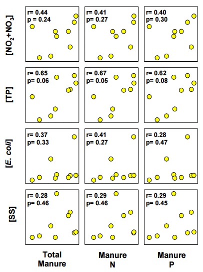
Relationships between stream water quality and manure production
Relating stream loads (2006-2009 average) of NO2+NO3, TP, E. coli, and SS to total manure production, manure N, and manure P produced in each watershed resulted in no statistically significant relationships, though the direction of these non-significant relationships were consistently in the positive direction (Figure 23). Interestingly, however, TP concentrations and total manure, as well as manure N, and manure P were statistically significant or marginally non-significant.
Comparison with PLUARG values
Mean precipitation across the Environment Canada stations in the region was 1002 mm in 1975 and 1040 mm in 1976, slightly higher than the mean precipitation we observed during the present work of 948 mm (see Patterns in Precipitation above).
While some of the PLUARG NO2+NO3 loading estimates were very similar to those of the present work, there were several notable exceptions (Table 15). In AG-03 (Figure 2), the PLUARG estimate at Little Ausable Creek of 2.6 × 10³ kg km-2 was remarkably similar to our estimate at the same stream of 2.5 × 10³ kg km-2. Our loading estimates at two of the three other streams in this region were also similar at 2.6 and 3.1 × 10³ kg km-2 at South Thames and Nineteen Creeks, respectively. Only at Silver Creek was loading of NO2+NO3 (4.4 × 10³ kg km-2) appreciably higher than at the other streams in the AG-03 region. Unlike NO2+NO3, estimates of TP loading in the AG-03 watershed varied widely. The PLUARG estimate of TP loading of 77 kg km-2 at Little Ausable Creek was roughly similar to our estimates of 54 kg km-2 at South Thames River and Nineteen Creek, respectively. However, our estimate of TP loading of 131 kg km-2 at Silver Creek was higher than the PLUARG estimate, and our estimate at Little Ausable Creek, the same AG-03 creek used in PLUARG, was higher still at 189 kg km-2. Suspended solids loading estimated at the Little Ausable River was 20 × 103 kg km-2, higher than our estimates at the South Thames River (12 × 103 kg km-2) and at Nineteen Creek (8 × 10³ kg km-2). As with TP, the SS loading estimates from our study were higher than the PLUARG estimate at Silver Creek (43 × 103 kg km-2) and the Little Ausable River (52 × 103 kg km-2).
There were three streams in the AG-04 watershed; Canagagigue Creek, studied during PLUARG, and the Avon and Middle Maitland Rivers, which were sampled for the present work. The NO2+NO3 loading estimate from the PLUARG work for Canagagigue Creek was 1.4 × 10³ kg km-2, which was lower than our estimate of 2.4 × 10³ kg km-2 of NO2+NO3 at the Avon River and appreciably lower than our estimate of 3.2 × 10³ kg km-2 at the Middle Maitland River. For TP, our estimate of loading at the Avon River of 89 kg km-2 was very similar to that the PLUARG estimate at Canagagigue Creek of 91 kg km-2. Loading of TP at the Middle Maitland River was appreciably higher than either the Avon River or Canagagigue Creek, at 167 × 103 kg km-2. However, our estimates of SS loading at both the Middle Maitland River and Avon River of 27 × 103 kg km-2 and 26 × 103 kg km-2 respectively, were lower than the PLUARG estimate of SS loading at Canagagigue Creek of 46 × 103kg km-2.
At AG-05, both the PLUARG study stream and our study stream was Nissouri Creek. Our estimate of NO2+NO3 loading at Nissouri Creek of 3.8 × 10³ kg km-2 was considerably higher than the PLUARG estimate of 2.3 × 10³ kg km-2. For TP, the PLUARG estimate of 81 kg km-2 was close to our estimate of 71 kg km-2. The PLUARG estimate of SS loading of 27 × 103 kg km-2 was approximately twice that of our estimate (13 × 103 kg km-2), however.
The PLUARG study stream at AG-06 was the Upper Maitland River, while our study streams were Blyth Brook and Muskrat Creek. The PLUARG estimate of NO2+NO3 loading was 1.2 × 10³ kg km-2, while our estimate at Muskrat Creek was similar at 1.8 × 10³ kg km-2 and at Blyth Brook our NO2+NO3 loading estimate was 2.3 × 10³ kg km-2. Our estimate of TP loading at Muskrat Creek (43 kg km-2) was more than twice that of the PLUARG estimate at the Upper Maitland River (16 kg km-2) though it was similar to the 20 kg km-2 of TP loading we estimated at Blyth Brook. The PLUARG estimate of SS loading at the Upper Maitland River of 6 × 10³ kg km-2 was the same as our estimate for SS loading at Blyth Brook, but substantially lower than SS loading at Muskrat Creek of 25 × 103 kg km-2.
| PLUARG region |
stream | NO2+NO3 (× 103 kg km-2) |
Comparison to reference |
TP (kg km-2) |
Comparison to reference |
SS (× 103 kg km-2) |
Comparison to reference |
|---|---|---|---|---|---|---|---|
| AG-03 | Little Ausable (PLUARG) |
2.6 | -- | 77 | -- | 20 | -- |
| AG-03 | Little Ausable | 2.5 | 1.0x | 189 | 2.5x | 52 | 2.6x |
| AG-03 | Silver | 4.4 | 1.7x | 131 | 1.7x | 43 | 2.2x |
| AG-03 | South Thames | 2.6 | 1.0x | 54 | 0.7x | 12 | 0.6x |
| AG-03 | Nineteen | 3.1 | 1.2x | 68 | 0.9x | 8 | 0.4x |
| AG-04 | Canagagigue (PLUARG) |
1.4 | -- | 91 | -- | 46 | -- |
| AG-04 | Avon | 2.4 | 1.7x | 89 | 1.0x | 26 | 0.6x |
| AG-04 | Middle Maitland | 3.2 | 2.3x | 167 | 1.8x | 27 | 0.6x |
| AG-05 | Nissouri (PLUARG) |
2.3 | -- | 81 | -- | 27 | -- |
| AG-05 | Nissouri | 3.8 | 1.6x | 71 | 0.9x | 13 | 0.5x |
| AG-06 | Upper Maitland (PLUARG) |
1.2 | -- | 16 | -- | 6 | -- |
| AG-06 | Blyth | 2.3 | 1.9x | 20 | 1.3x | 6 | 1.0x |
| AG-06 | Muskrat | 1.8 | 1.5x | 43 | 2.7x | 25 | 4.2x |
Discussion
Comparison to larger watersheds and the region as a whole
We compared NO3- and TP concentrations in the study streams to the concentrations of these measures in other streams in the same major watershed (monitored as part of the PWQMN) to provide a general context for the concentrations we found in the study streams. Concentrations of NO3- were generally higher (albeit this was often slight) in the study streams than for other streams in the same major watershed. Concentrations of TP showed more variability in comparison to the general PWQMN, with some streams having much higher median TP concentrations than their respective reference watersheds. The PWQMN sites we compared our study streams to are typically on larger streams than those of the present study. The streams of the PWQMN would also have more varied influences in their watersheds, rather than the agricultural dominance of the watersheds in the present study. Comparisons to the streams in our study should be made with these perspectives.
With these varied influences aside, small streams in agricultural regions have been found to have higher nutrient concentrations than the streams that they drain into for several reasons. Firstly, small streams, such as our study streams, are important sites of nutrient transformation. Alexander, Smith, & Schwarz (2000) found that nitrogen removal rates were far higher in small streams than in the larger streams collecting these inputs. They concluded that proximity of sources to large streams was important in determining stream nitrogen concentrations. A similar finding has been made for phosphorus removal in streams (McDowell et al. 2004). Thus, small streams, such as those in the present study, are likely important in reducing the amount of nitrogen and phosphorus delivered to larger receiving streams.
The concentrations of TP in the study streams were also more variable that those measured in their larger watersheds. This greater variability in TP concentrations is likely because TP has a large sediment-bound fraction. Thus, streams, or reaches of streams, can be high in TP from high inputs from land use, high erosion in the watershed or stream banks, or an erosive flow regime. Conversely, TP can also be lost from the water column by a sedimenting flow regime. Additionally, since phosphorus is typically the limiting nutrient in freshwaters, the more labile fractions of TP can also be lost from the water column through rapid uptake by stream biota.
Comparison to pre-impact loading and concentration estimates
The study region as a whole is under considerable human influence. Thus, extant pre-anthropogenic impact baseline values are not available. Streams that are minimally impacted are available on the periphery of the study area. However, these areas are minimally impacted because they are inherently different (e.g. poor agricultural land) so would not necessarily serve as adequate non-impacted references. Work done by the National Agri-Environmental Standards Initiative (NAESI) has estimated pre-impact (i.e. prior to anthropogenic influence) concentrations for TN and TP in Southern Ontario using five different approaches (Chambers et al. 2009). These pre-impact concentration estimates were then used to generate an “Ideal Performance Standard” (IPS) for several regions in Canada, including the “mixed hardwood region on Ontario”, which encompasses our study region. The IPS is defined as, “the desired level of environmental quality needed to maintain ecosystem health” (Chambers et al. 2009). The NAESI estimate for the pre-impact levels of TP for the mixed hardwood region ranged from 8 to 32 µg L-1, depending on the method used. For TN, the pre-impact estimates ranged from 0.24 to 1.31 mg L-1.
Using these estimates of pre-impact TN and TP concentrations, NAESI developed an IPS of 24 µg L-1 for TP and 1.07 mg L-1 for TN for the mixed hardwood region of Ontario. Note that for these studies the authors determined TN, rather than NO2+NO3concentrations as we determined in this work. However, NO2+NO3 comprised 80-90% of the TN in our study. Thus, for comparison purposes, we compare the TN IPS concentrations of NAESI to the NO2+NO3 concentrations generated in the present study. The TWMC for NO2+NO3 across streams for which we could derive such data was 6.2 mg L-1, which is 5.8 times higher than the TN IPS values estimated by NAESI. For TP, we estimated a TWMC of 60 µg L-1, 2.5 times higher than the TP IPS values estimated by NAESI. Thus, nitrogen concentrations are more elevated compared to the NAESI IPS than are TP concentrations.
One consideration in the interpretation of TP concentrations relative to estimated pre-impact concentrations and IPS values is the relative lability of TP fractions. Stream TP is largely sediment-bound and biologically unavailable (e.g. Logan 1982). Against a background of a large amount of recalcitrant P, a quantitatively small input of highly labile P might be an undetectable fraction of TP. However, this small input could represent a substantial increase in the proportion of available P in the system. Unfortunately, the proportion of labile P is difficult to measure and currently no routine measures of biologically available P are available. Focussed studies on the fraction of labile P, perhaps in a subset of these systems, may help quantify the contemporary proportion of labile P in these streams.
The NAESI work concedes that the IPS is not likely to be achievable in areas of appreciable agricultural influence. Thus, the NAESI also identified “Achievable Performance Standards” (APS), their estimate of concentrations that can be achieved using recommended beneficial management practices. The APS are site-specific and they were derived for particular watersheds in the NAESI study using watershed-modelling techniques. For example, NAESI developed APS for the Raisin River in Eastern Ontario. At the outlet of the Raisin River, modelling done by NAESI estimated that 20m buffer strips along the river have the potential to reduce TN from 3.37 mg L-1 to 1.78 mg L-1 and reduce TP from 113 µg L-1 to 31 µg L-1 (Chambers et al. 2009).
As we alluded to earlier, the effect of BMPs, and therefore the APS, will be watershed specific. Thus, we currently cannot identify APS objectives for our study sites. However, work currently underway by our branch, is modelling the potential impact of BMPs on Nissouri Creek. Additionally, our group is involved in a project that is funded by OMAFRA under the Canada-Ontario Agreement known as the Watershed Based Best Management Practices Evaluation (WBBE) Program. This project will also model the potential improvements in water quality with the application of various BMPs in a variety of watersheds in Southwestern Ontario.
A NAESI subproject developed some estimates for unimpacted (from human influence) E. coli concentrations (Edge et al. 2009) and applied these values as provisional standards for E. coli in agricultural regions. In this work, the authors developed estimates of the concentration of E. coli that corresponded to background diversity of waterborne pathogens (Cryptosporidium, Campylobacter, and Giardia) by using minimally impacted upstream reaches of their study watersheds in a variety of locations across Canada. Edge et al. (2009) found that the background levels of E. coli depended on stream order, with unimpacted streams of higher order showing lower concentrations of E. coli than lower-order unimpacted streams. Specifically, they determined that for third-order and lower streams, unimpacted reaches of their study streams had mean annual E. coliconcentrations < 84 CFU 100 mL-1. For streams higher than third-order, they found that unimpacted streams had mean annual E. coli concentrations < 39 CFU 100 mL-1. These two values were used as the provisional standards for streams of third order or lower, and for streams of greater than third-order, respectively.
In the present study, the streams ranged from second to fifth order. For the second and third-order streams (Blyth Brook, Muskrat Creek, the Middle Maitland River, Nineteen Mile Creek, and Silver Creek), the TWMC of E. coli that we estimated over the course of the study was 893 CFU 100 mL-1, approximately ten times higher than the NAESI provisional standard of < 84 CFU 100 mL-1. The range in average values for these streams varied considerably, however, from 149 CFU 100 mL-1 at Nineteen Mile Creek, to 2500 CFU 100 mL-1 at the Middle Maitland River. For the fourth- and fifth-order streams (Nissouri Creek, the Avon, Little Ausable, and South Thames Rivers), our computed average TWMC for E. coli was 403 CFU 100 mL-1. As with the lower-order streams, this value was approximately ten times greater than the NAESI provisional standard for streams greater than third-order. None of the streams for which we have TWMC data were below the NAESI provisional standards in the 2006-2009 average E. coli concentration. For the larger set of streams which was sampled, but for which we could not generate TWMC, the mean value across all streams of 1425 CFU 100 mL was well above the NAESI provisional standards.
Estimates for the pre-impact loads or concentrations of SS do not exist for our study area. While agriculture often has impacts on erosion and the subsequent sediment loading in streams, it is likely difficult to generate estimates for pre-impact loads or concentrations as some pristine streams can, at least periodically, can generate high loadings of SS due to natural erosion. Thus, natural SS loading and concentration likely vary greatly among streams.
Pre-impact nutrient loading estimates are not available for Ontario. However, Smith, Alexander & Schwarz (2003) generated pre-impact loading estimates, on a regional basis, for the conterminous United States. To provide some basis for comparison, we compare our values to reference values calculated for regions in the US that are adjacent to the study region in the present study. As with the values for the NAESI project, Smith, Alexander & Schwarz (2003) determined TN, rather than NO2+NO3 concentrations, though we shall compare directly our NO2+NO3 loading estimates. Thus, the TN loading estimates will represent a slight overestimate compared to NO2+NO3 loadings. For the “Corn Belt and Northern Great Plains”, a region adjacent to the part of the western shore of lake Huron and part of the southern border of Lake Erie, they estimated median pre-impact loadings of TP of 7.3 kg km-2 y-1, and TN loadings of 60 kg km-2 y-1. For the “Mostly Glaciated Dairy Region” also partially adjacent to the western shore of Lake Huron, as well as part of the southern border of Lake Erie, they estimated similar pre-impact TP loadings of 6.2 kg km-2 y-1, and TN loading of 70 kg km-2 y-1. Our average NO2+NO3loading was 3.1 × 10³ kg km-2 y-1, which ranges from 44 to 52 times that of the pre-impact loadings estimated by Smith, Alexander & Schwarz (2003). For TP, our average estimate of loading was 92 kg km-2 y-1, approximately 12 to 15 times higher than the estimates of Smith, Alexander & Schwarz (2003). Thus, as with the comparison of concentrations against the NAESI IPS, it would appear that nitrogen loadings are further above pre-impact levels than are phosphorus loadings.
Because the loading estimates of Smith, Alexander & Schwarz (2003) are only adjacent to the study area of the present study, it is possible that they do not reflect pre-impact loadings for the study area. However, in the same study, Smith, Alexander & Schwarz (2003) also estimated pre-impact concentrations regionally, and those pre-impact concentrations for the Corn Belt and Northern Great Plains and the Mostly Glaciated Dairy Region are similar to the pre-impact concentrations of TN and TP generated in the NAESI study, suggesting that pre-impact loading might also be similar in these adjacent regions. An estimate of pre-impact loadings for Southwestern Ontario, nevertheless, would result comparisons for our study region that are more robust.
Relationships within the study watersheds
While the percentage of agriculture in the study watersheds varied in a relatively small range, from 64 to 95%, NO2+NO3 unit-area loadings varied 3-fold. This finding is consistent with a study done by Caraco et al. (2003). They found that in large rivers, NO3- export was well explained by simple measures of human activity. On smaller watersheds (< 100 km-2), however, this relationship weakened, predicting only 8% of the variation in NO3- export even though the range in NO3- export in their data was > 1000 fold. As all of our watersheds are under 100 km-2, with some considerably smaller than this, it is perhaps not surprising that the variability in a coarse measure of land use does not correspond with the degree of variability we observe in NO2+NO3 loading among our watersheds. Caraco et al. (2003) indicate that patterns explaining NO3 export, especially in small watersheds, are resolvable with more detailed land use information. As mentioned, we are currently seeking to obtain data of sufficient detail to explain more fully the variability we observe in NO2+NO3 loadings among these watersheds.
The range in TP, SS, and E. coli loadings were even greater than that of NO2+NO3, with TP and SS loadings ranging close to an order of magnitude difference and E. coli almost two orders of magnitude among streams. The reason for this difference in the range of these water quality measures among streams is likely due, at least in part, to solubility differences. Of these water quality measures, NO2+NO3 are the only forms that are entirely soluble. Suspended solids, as their name implies, are insoluble and tend to be transported in far greater quantity during high-flow, rather than low-flow periods. The amount of SS transported by a stream is highly dependent on soil type and stream morphology, so variability in these could contribute to additional variability among the streams. Total phosphorus presents a further complication in that fractions of TP are highly soluble, while other fractions (typically the majority in streams) are insoluble, with a range of colloidal and semi-soluble P fractions as well. The sediment-bound insoluble fraction, like SS, is exported in much larger quantities during high-flow events (Logan 1982). E. coli, while minute in size, tend to bind to much larger sediment particles. Thus, like TP, E. coli tend to travel with SS. Additionally, E. coli typically are highly variable, both temporally and spatially within streams.
Comparison to PLUARG
There are several considerations to remain aware of when comparing our loading estimate to those of the PLUARG work completed over 30 years ago. The PLUARG values are means of two study years (1975 and 1976) and our values are the means of 4 to 6 years of study. As described earlier, weather-driven year-to-year fluctuations in stream loading can be appreciable, so our snapshot comparisons could be strongly influenced by such fluctuations. Annual precipitation in the PLUARG study years and the study years of the present work did not differ greatly, however. These annual means do not consider the potentially important influence of within-year patterns in precipitation (such as the frequency of storms), so climatic differences cannot be entirely excluded as a consideration in comparing these studies. Two of our streams were also examined in the PLUARG work (the Little Ausable River and Nissouri Creek) while we grouped the remainder of our streams by the sub-watersheds identified by the PLUARG. The PLUARG sub- watersheds were chosen to have similar soil types and land uses (see Methods). However, appreciable variation in soil types and land use occurs in these watersheds, so it is quite likely that streams within the PLUARG regions would display considerable variation in water quality due to these differences. Another consideration in making comparisons between the loading estimates of the present work and those of PLUARG are the loading estimates themselves. The PLUARG work was able to sample far more frequently (> 1 sample per day on average) than in our study design (see Methods). While the NO2+NO3 loading estimates are likely comparable between our work and that of the PLUARG, we expect that our calculations of TP and SS loadings are underestimates compared to those of the PLUARG work (see “Methods- Comparison with PLUARG values”).
While all of the above considerations must be kept in mind when comparing our loading estimates to those of the PLUARG work, some of the comparisons between our work and those of the PLUARG remain remarkable. One such stream is the Little Ausable River, which was studied by the PLUARG as well as in the present work. This stream showed much higher loadings of TP and SS in our work than that found by the PLUARG (2.5 and 2.6 times, respectively). Our estimates of TP and SS loadings at Muskrat Creek were also much higher than at the PLUARG reference site (Upper Maitland River), where TP loads were 2.7 times and SS loads were 4.2 times higher than that of the Upper Maitland River. More intensive sampling using automated sampling to capture high-flow events would improve our estimates of loading at these streams.
Remarkably higher loadings were not only evident in TP and SS, as several of our estimates of NO2+NO3 loading were much higher than that estimated by the PLUARG. Silver Creek, in the same PLUARG region as the Little Ausable River (AG-03), showed high loadings of TP and SS, but also had appreciably higher NO2+NO3 loadings than those estimated by the work of the PLUARG on the Little Ausable River. The Middle Maitland River, examined in the present work, had NO2+NO3 loads 2.3 times higher than the reference stream studied by the PLUARG for that region (Canagagigue Creek). The loading of TP was also high at The Middle Maitland River at 1.8 times that the PLUARG reference. Curiously, our estimate of SS loading at the Middle Maitland River was only 0.6 times that of the PLUARG reference. This finding is remarkable because TP tends to be sediment-bound, so an increase in TP loading is unexpected without a concomitant increase in SS loadings.
Our estimates of NO2+NO3 loadings at Nissouri Creek, which was also studied by the PLUARG, were appreciably higher than the estimates that their work generated. Loadings of TP between our study and that of PLUARG were similar, and our estimate of SS loading was only half that of the PLUARG work. Again, it is important to consider that our estimates of SS and TP loading are likely underestimates compared to the PLUARG estimates.
Recent estimates of stream loading at Nissouri Creek have also been generated in a study by the Ontario Ministry of Farm and Rural Affairs (OMAFRA) and the Soil Resource Group (SRG 2010). For Nissouri Creek, estimates of NO2+NO3loading in this study (average of 2008 and 2009) were similar to our estimate (3.4 × 10³ kg km-2 y-1 compared to our estimate of 3.8 × 10³ kg km-2 y-1). However, estimates of TP and SS loading by the OMAFRA and SRG work at Nissouri Creek are substantially higher than our estimates. For TP, the OMAFRA and SRG estimate is 190 kg km-2 y-1, while our estimate is only 71 kg km-2 y-1. Similarly, the OMAFRA and SRG study found SS loadings of 39 × 103 kg km-2 y-1, while our estimate is only 13 kg km-2 y-1. These results corroborate our earlier supposition that our sampling frequency results in an underestimate of TP and SS loads and suggest that loadings of all of these substances were appreciably higher between the late 1970s/early 1980s and the recent past in the Nissouri Creek watershed.
The OMAFRA/SRG (2010) study also estimated stream loading at Canagagigue Creek at the same site as that of the PLUARG work. Similar to their findings at Nissouri Creek, average annual loadings of NO3- increased appreciably between their study years (2008 and 2009) of 2.9× 10³ kg km-2 y-1 versus those of PLUARG at 1.4× 10³ kg km-2 y-1. TP and SS loadings between the two periods did not appear to have changed greatly at the Canagagigue watershed, however. Their study estimated TP loadings of 100 kg km-2 y-1 compared to 90 kg km-2 y-1 found by PLUARG. Similarly, the OMAFRA/SRG study estimated SS loadings of 30 × 103 kg km-2 y-1, while the estimate during the PLUARG study was 46 × 103 kg km-2 y-1. Our findings, and those of the OMAFRA/SRG (2010) work, suggest that loadings of some substances at some watersheds have increased but also suggest that there is appreciable variability in the changes in water quality among streams.
Seasonal loads and concentrations
Perhaps the most striking feature that we observed in the seasonal pattern in stream loads and concentrations was the relatively high winter concentrations and loads of TP, NO2+NO3, and SS. As demonstrated in Figure 7, rather than a spring thaw occurring in March, winters were typically marked by several thaw events, often accompanied by rain. A high proportion of these snowmelts and winter rains contributed to increased discharge during this time of year when rates of evapotranspiration and infiltration (due to frozen soils) are low. Indeed, a large portion of annual discharge (41%) occurs in the 3 winter months. Work done by the PLUARG found a similar proportion of winter stream loading in their study of agricultural watersheds in Southwestern Ontario (Ongley 1978).
For NO2+NO3, the seasonal proportion of loading was very closely related to the proportion of discharge in that season (and each of the other seasons). The NO2+NO3 relationships with discharge were also simple in that high NO2+NO3 loading in winter corresponded with high NO2+NO3 in-stream concentrations. For TP and SS, the proportion of winter loads was slightly higher than the proportion of discharge delivered in the period. Additionally, the concentration/loading relationship was somewhat more complicated, with high loads of TP and SS not always resulting in correspondingly high concentrations. This is probably because winter discharge was dominated by high-flow events, which would likely result in relatively more erosion during these winter flows. Erosive events would result in periodically high loading, but lower flows during winter would mean that, for the intervening low flow periods, TP and SS concentrations would be relatively low.
Concerning in-stream effects, the cold temperatures could mute some of the potential effects of high concentrations in winter and late autumn. Biological activity would be relatively low during this time of year. Thus, the in-stream eutrophication potential of increased TP is likely to be much lower than the potential effect during warmer times of the year. The relatively lower biological activity might also result in lower toxicity of NO2+NO3 to stream organisms at low temperatures. One of the mechanisms by which nitrite (NO2-), the more toxic form of the two, exerts much of its toxicity on aquatic organisms by interfering with oxygen metabolism (Jensen 2003). Oxygen concentrations are typically higher in winter, which could mitigate some of the toxicity from NO2- though with low flows and under ice cover, high oxygen concentrations in winter might not always be the case (Gordon 2004). Studies relating the toxicity of NO2 or NO3- with temperature are sparse. It has been found in channel catfish that lower temperatures resulted in slower development of NO2 toxicity, likely due to lower respiration rates (Lewis & Morris 1986). However, the same work found that lower temperatures also result in lower rates of detoxification of NO2--. Thus, the ecological implications of high NO2+NO3 concentrations in winter are currently unclear.
The relatively high winter concentrations and loads of TP, NO2+NO3, and SS that we observed could have important implications for receiving waters, where these waters receive inputs from agricultural streams similar to our study streams. For example, high winter NO2+NO3 loads from agricultural streams could contribute to elevated NO2+NO3 concentrations at drinking water intakes located in downstream receiving waters, including nearshore regions in the Great Lakes. Further study would likely reveal if the seasonal patterns we observe in these small agricultural streams were reflected in receiving waters.
Nutrient loads, especially TP, which are delivered to the Great Lakes in winter, have the potential of resulting in eutrophication issues in spring, if these inputs are held close to shoreline over the winter. The fate of riverine inputs during winter is poorly understood. However, it is plausible that shoreline ice, followed by thermal bar formation in spring, could hold TP and NO2+NO3 delivered by rivers close to the shoreline long enough to result in eutrophication issues in early spring. Nearshore studies on the South East shores of Lake Huron have found some evidence of spring elevation in algal growth that is not clearly linked to a current river input (Mohamed, Howell, & Todd 2009). It is possible, though not confirmed, that these increases were the result of winter loading from adjacent streams that were trapped in the nearshore until spring temperatures increase.
While the loads and concentrations of NO2+NO3, TP, and SS were highest in winter, spring loads (March-May) and concentrations of these were also high, to varying extents. Indeed, SS concentrations peaked during March. Increasing temperatures at this time of year would increase the potential for both in-stream as well as nearshore eutrophication from TP inputs. The NO2+NO3 loadings, which also remain high for this period, potentially present the same issues for receiving waters as described above.
Figure 24: Discharge of the Maitland River near Lake Huron (grey) and NO2+NO3 concentration at the Goderich drinking water intake (blue) from 2004 to 2009. NO2+NO3 data from The Great Lakes water intake monitoring programme, discharge data from Hydat gauge at Benmiller. Note that water quality samples were not collected from February 27 to June 5, 2006.
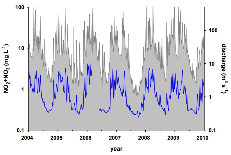
By late spring, loading and concentration of TP, NO2+NO3, and SS dropped, to varying extents. In the case of NO2+NO3, both the loadings and concentrations were very low in summer compared to the other seasons. While the larger receiving rivers would also have other inputs of NO2+NO3, previous work on large rivers in Southwestern Ontario, including the Bayfield, Maitland, and Saugeen Rivers, show that these rivers display the same pattern of high NO2+NO3 concentrations in late autumn and winter, and much lower NO2+NO3 concentrations in summer (Mohamed, Howell, & Todd 2009). Additionally, at the Goderich drinking water intake, close to the outlet of the Maitland River, the same pattern of NO2+NO3 inputs to the adjacent shores in the nearshore of Lake Huron can be observed (Figure 24).
In the case of TP loads and concentrations, an interesting seasonal pattern emerged. While loads of TP decreased, concentrations increased in July, remaining above the monthly average for the summer. During this period, flow generally decreased to very low levels, often becoming close to stagnant in many of the study streams. Thus, while TP concentrations can remain high, loading of TP during these periods would be very low.
The TP concentrations during low flows could have considerable consequences for stream biota and chemistry. The growth of attached and planktonic algae in the study stream is likely limited by P. During low-flow, extended periods of high P concentration could therefore allow growth of attached or planktonic algae. Low flow also results in lower rates of oxygen exchange with the atmosphere. During nights, high biomass of attached or planktonic algae, and their potential consumers could result in appreciable respiration, potentially reducing oxygen concentrations on a diel cycle. Previous work at the Middle Maitland River showed that oxygen concentrations dropped to very low concentrations on a diel basis (Clerk 2007). These low oxygen concentrations could have detrimental effects on some stream biota. Additionally, low flows coupled with reduced oxygen in the overlying water could also result in sediment anoxia, a process that can release P from bottom sediments.
While loading of TP in summer was relatively low, it is also important to consider that discharge in receiving streams would also be low during summer. Thus, the high summer TP concentrations could also result in high concentrations in the receiving streams. While daily estimates of load or concentration were not determined in the study by Mohamed, Howell, & Todd (2009), it was found that TP concentrations were generally lower in three large rivers draining Southwestern Ontario into Lake Huron during the summer. However, TP concentrations periodically did increase appreciably during summers. In the Grand River, Jamieson (2010) and Rosamond et al. (2011) found that nutrient inputs from agricultural as well as municipal sources resulted in high stream respiration, which, in turn resulted in diel depletion of oxygen concentration in the river.
E. coli concentration and loading was different compared to nutrients and SS, particularly in the winter and spring, which was likely related to different transport potential and survival rates at these times of year. While E. coli loads increased in early autumn, they declined in late autumn and remained low throughout winter and spring. A similar pattern was noted by Donnison, Ross, & Thorrold (2004) in New Zealand streams. In the streams of the present study, this pattern could probably be attributed, at least in part, by colder weather resulting in the die-off of E. coli. However, Hunter et al. (1999) related the pattern of stream E. coli concentrations to animal stocking rates in the associated watersheds, while Hunter & McDonald (1991) attributed the late season depletion of E. coli to their washout from the surrounding land by frequent autumn and winter rainfall.
Since E. coli loadings were highest in early autumn, this is possibly when the greatest impacts to receiving waters would occur. As with TP, however, receiving streams are also likely to have lower flows in summer potentially resulting in high E. coli concentrations in receiving waters during summer. Mohamed, Howell, & Todd (2009) noted that, as with TP, E. coli concentrations during summer were generally low, but did periodically increase appreciably, especially in the smallest of the three rivers (Bayfield River). To confirm this pattern, further work on the seasonal pattern of E. coli would have to be done on these larger receiving waters.
Seasonal loads and land management
As described above, the PLUARG work found that a majority of the nutrient loads arrived to their study streams in autumn to early spring (Neilsen, Culley, & Cameron 1978). The authors note that the lack of plant growth in the watershed from November to April, coupled with low denitrification rates due to low temperatures (Kowalenko 1978) resulted in large leaching losses from the soil. They recommended that efforts directed at reducing the nitrate content of soil prior to autumn would result in significantly lower annual loading of nitrogen to streams. They also recommend the planting of autumn cover crops to immobilise nitrogen as plant biomass or an organic (and therefore less soluble) form of nitrogen to decrease nitrogen loadings.
More recently, studies in other agricultural regions have come to some similar conclusions. In a study of the movement of nitrogen fertilisers through corn crops, Sanchez & Blackmer (1988) found that 49-64% of fertiliser N applied in autumn was lost from the upper portion of the soil, primarily in the autumn to spring period. Similarly, a review by Dinnes et al. (2002) stated that a key factor in reducing N losses from soils was to limit the amount of N within the soil at the end of the growing season and before the next season’s crop has established an extensive root system. In Sweden, an examination of possible policy measures to reduce nitrate leaching at the watershed scale recommended, among other measures, the planting of winter crops to reduce nitrate leaching (Gustafson, Fleischer, & Joelsson 2000), as well as ceasing autumn fertiliser application (Hoffman & Johnsson 2000). In Denmark, appreciable reductions in the amount of surplus nitrogen and phosphorus in soils have been achieved through a combination of setting upper limits for animal density and soil nitrogen, as well as restriction on winter application of manure (Maguire et al. 2005; Schelde et al. 2006). Lewis & Makarewicz (2009) applied a suite of BMPs, including restriction of winter manure spreading, to a small watershed (Graywood Gully). After 3 years, they resumed winter manure application as the sole change to the suite of BMPs employed. Within a short period, they found a dramatic increase in TP, NO3-, total kjeldahl nitrogen, and soluble reactive phosphorus in the stream draining the watershed. They recommended that, to reduce macrophytes in a downstream lake (Lake Conesus), reduction of winter loading was of key importance.
As noted above, the PLUARG studies done over 30 years ago found similar seasonal patterns in stream loading, with winter and early spring loadings dominating annual loads of nutrients and SS (Ongley 1978). Land use practices in the province have changed appreciably in the intervening period. For example, winter spreading of manure is no longer recommended and there are several restrictions on the winter application of agricultural source materials, including manure (though it is not prohibited; O. Reg. 267/03). It is notable, therefore, that the seasonal pattern in stream loadings of nutrients and SS remain similar between our study and that of the PLUARG. Further work to elucidate the mechanisms resulting in high winter loadings of NO2+NO3 in these watersheds is warranted.
Inter-annual patterns in loading
As outlined in the Methods and Results, we generated a single loading model across years for each stream. Thus, the year-to-year differences in loading estimates are based on the same relationship between concentration and discharge. The inter-annual patterns, however, demonstrate the degree to which loadings in a single year are affected by variation in weather. In 2007, a relatively dry year, loadings of all water quality measures in all streams dropped dramatically. The following year was relatively wet, resulting in a dramatic increase in loadings for all parameters. The strong dependence of annual loading rates on precipitation is an important consideration in the interpretation of trends and their potential relationship to land use and management practices. For example, in a simulation of nitrate export in a Minnesota stream, Nangia, Mulla, & Gowda (2010) found that precipitation had a greater effect on nitrate export than did changes in land management practices for three periods from 1965 to 2003. Thus, interpretation of temporal trends, especially short-term trends, should be made with great caution and apparent changes among years should be compared to other streams. A combination of monitoring and experimental approaches would likely result in the most robust evaluation of the effects of land management changes on stream water quality.
Climate effects and implications
The importance of inter-annual variations in weather demonstrated above also suggests that climate change could have an effect on stream nutrient loading and water quality. In a study of historical stream data in Ohio, Moog & Whiting (2002) found that the majority of the increase in stream loading from 1976-1995 was not from changes in land use, but rather due to climatic factors. Their analysis determined that increases in winter stream flow and the associated decrease in snowfall and snow cover were responsible for increases in NO2+NO3 and SS loads, while only soluble reactive phosphorus was increased from changes in agricultural practices. These findings suggest that it is possible that the high winter loading we observe in our study streams could be enhanced with climate change if such change were to increase the number of thaw events and decrease snow cover during winters. It is likely that the effect of climate change on stream nutrient loads will have considerable spatial heterogeneity, with different locales showing very different responses. For example, Chang, Evans, & Easterling (2001) conducted a simulation of changing stream flow and nutrient loading under a climate change scenario with an assumption of no change in land cover and land management in six watersheds of the Susquehanna River Basin. They found that stream flow and nutrient loads increased for most watersheds, but decreased in one intensively cultivated watershed. For our study streams, and Southwestern Ontario in general, understanding the potential impact of climate change will require specific studies to separate the effects of climate from land use, as well as to project possible future changes from the combined effect of changes in land use and climate.
Patterns in base flow
Our estimates of base flow contribution were done through numerical analysis of stream hydrographs and were not field calibrated. Thus, the per cent base flow estimates could vary appreciably from actual values. However, we applied the same techniques to all streams and the estimates serve as a relative measure of base flow contribution to the study streams. A thorough examination of the relative contributions of base flow to stream loads is beyond the scope of this work. We are currently in the process of completing detailed analyses of base flow relationships and their implications to agricultural inputs in these streams. Some notable early observations are discussed below.
The per cent of flow attributable to base flow varied considerably, from 46% to 72% of stream flow, when averaged across study years for each stream. This variability likely affects how these streams respond to inputs. TP and SS move primarily by overland transport (e.g. Gburek & Sharpley, 1998) while NO2+NO3 have a larger component that moves through base flow and interflow (Green et al. 2007). These variable pathways can have implications for the type of management practices used to reduce nutrient loss to streams. In a stream with low base flow, BMPs to reduce erosion and surface runoff during storms might be the most effective strategies to reduce the transport of nutrients to the stream from surrounding land. For example, the Little Ausable River has low base flow and high loading of TP, SS, and E. coli, though its loadings of NO2+NO3 are not especially high when compared to the other study streams. Thus, strategies to reduce runoff and erosion might be the most effective in reducing loading of these substances at the Little Ausable River. Of course, the nature of the agricultural inputs, as well as other soil and geological characteristics affect the loss pathways of agricultural effluents and these must be considered based on the individual watershed.
Another example of how the proportion of base flow among the watersheds might affect the timing of the delivery of nutrients to streams can be observed in some of the exceedance data. As noted previously, the Middle Maitland River produced relatively high loads and concentrations of NO2+NO3 among watersheds. However, this stream had the lowest number of exceedances of NO3- among any of the watersheds from 2004-2009. Conversely, Muskrat Creek had a relatively high rate of NO3- exceedance, even though it had among the lowest loads and average concentration of NO2+NO3 among the study streams. These differences might be attributable to the higher proportion of base flow in Muskrat Creek, which would result in more stable flows than in the Middle Maitland River, which would have a comparatively more variable flow regime. The relatively high per cent base flow of Muskrat Creek, however, could result in concentrations consistently in exceedance of a given benchmark, even though the average load delivered was lower than a stream with a more variable flow regime, such as the Maitland River.
Across streams, the proportion of base flow increased in summer and decreased in winter. Loading of most water quality measures (aside from E. coli) followed the opposite pattern – increasing in winter and decreasing in summer. Ostensibly, these results suggest that the high winter loads are not due to high base flow load. However, high flows increase both the base flow as well as quick flow (e.g. Figure 7). Further analyses, separating the base flow contributions from quick flow, could reveal if there are seasonal patterns in the load arriving through the base flow.
Figure 25: A) Monthly variations in the base flow enrichment ratio found by Schilling and Zhang (2004) in the Racoon River with generalised seasonal pattern of nitrogen uptake by corn (arbitrary scale).
B) Monthly pattern in NO2+NO3 concentration and loading in the study streams, with a generalised seasonal pattern of nitrogen uptake by corn (blue points). Corn uptake pattern modified from Schilling and Zhang (2004).
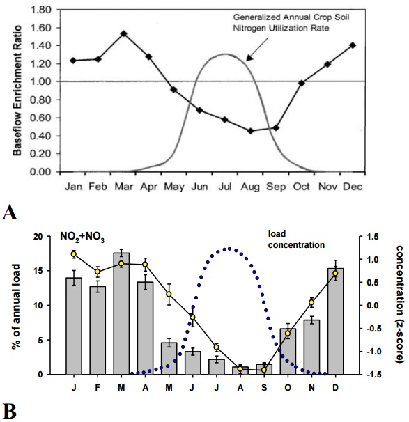
The proportion of stream flow attributable to base flow could also be used to determine what types of BMPs will be the most effective in different watersheds. For example, in the examination of a large agricultural watershed in Iowa (the Racoon River), Schilling & Zhang (2004) developed a method to determine the degree to which base flow concentrations of nitrate were enriched compared to total stream flow (base flow enrichment ratio, or BER). They found that the BER was high in this watershed, and was higher in winter than in summer (Figure 25A). Similarly, Dinnes et al. (2002) demonstrated that base flow loss of NO2+NO3 is much greater at times of the year when crop uptake is low. Note that the pattern in total NO2+NO3 load and concentration that we found (Figure 25B) is strikingly similar to that found by Schilling & Zhang (2004), who concluded the high winter BER of NO2+NO3 was due to low plant uptake of NO2+NO3 during winter. For the Racoon River watershed, Schilling and Zhang recommended BMPs to reduce base flow delivery of NO2+NO3such as improved riparian zone management, introduction of strategically-placed wetlands, or modifying drainage control structures. Further analyses of base flow data from our streams have the potential of revealing whether BER of NO2+NO3 in our study streams is also increased in winter, and whether this varies among our study streams. Such findings might help in determining the type of BMPs that would be effective in reducing entry of nutrients to the various streams.
Land use and its influence on loads and concentrations
The land use data are of a general nature and exclude important variables (e.g. quantities of fertiliser applied). We also do not quantitatively consider the potential effects of wildlife sources of nutrients and E. coli in these watersheds. Microbial source tracking studies have found that the E. coli found in streams and beaches draining agriculturally-dominated regions were primarily from a livestock, rather than wildlife, source. For example, Kon et al. (2009) found that, in recreational waters of the Lake Huron shoreline (close to the study region of the present work), the majority of E. coli were strains from livestock. Similarly, Graves et al. (2007) demonstrated that, in a livestock dominated region of Virginia, cattle were the dominant source of E. coli. Additionally, Graves et al. (2007) determined that cattle-derived strains of E. coli remained the dominant source regardless of season or sampling location within the study watershed. It remains a speculative possibility that wildlife could provide an appreciable source of nutrients or E. coli if appreciable upstream habitat were present. Most of our study watersheds however, have few, if any upstream sources of standing water. A potential exception to this is the Avon River watershed, which has a few small upstream ponds created by artificial dams. Notably, the E. coli, nutrient, and SS concentrations at the Avon River sampling site, do not appear anomalous compared to our other study watersheds.
While the above caveats must be considered, our land use data do provide some important characteristics of watersheds and some of the broad patterns between land use and stream water quality were evident. Generally, we found a pattern of increasing crop and livestock densities that were related to increased TP, NO2+NO3 and E. coli concentrations as suggested by the redundancy analysis. Individual correlations between cattle and poultry densities and water quality were sometimes statistically significant, though the relationships were generally weak. A seemingly anomalous observation in the relationship between land use and water quality (Figure 22) was the lack of relationship between pig density and any of the water quality variables. This, however, is likely due to sampling artefact. In the full dataset of 15 streams, there were positive relationships between cattle, pig, and poultry densities (Figure 5). The positive relationship between cattle and poultry density also occurs in the smaller set of 10 streams for which we have loading data. However, in that smaller set of streams, there is no positive relationship between pig and cattle densities, or pig and poultry densities. Thus, for this smaller dataset, pig density was uncorrelated to poultry and cattle densities, and therefore also appeared to be unrelated to TP, E. coli, and NO2+NO3 concentrations. This is most likely only a reflection of small number of sites we had available for generating stream loads (and thus TWMC).
Another interesting observation we made when relating land use to water quality was that soybean density was negatively related to TP, NO2+NO3, and E. coli concentrations. In terms of land use variables, soybean density was positively related to increasing per cent base flow and negatively related to cattle and poultry densities, both of which loaded in the same direction as E. coli, NO2+NO3, and TP (Figure 22). Thus, in our dataset, regions of greater soybean farming were regions of low livestock densities and were also regions that had a higher proportion of base flow and less impacted water quality. Consequently, it is likely that higher soybean density was associated with lower TP, NO2+NO3, and E. coli because regions of high soybean density were regions of low livestock density. Whether this pattern holds for the larger region and its causality, however, are beyond the scope of this work. Interestingly, work done by the PLUARG project on soil nitrogen losses under different cropping practices found that most crop types (tobacco, corn, winter wheat, potatoes, and green beans) produced a considerable amount of leachable N. Soybean however, did not (Neilsen, Culley, & Cameron 1978).
Many of the qualitative relationships between land use and stream water quality in individual streams were interesting, if not entirely explicable. For example, the Middle Maitland River showed high loading and concentrations of NO2+NO3, TP, and E. coli. The watershed of this stream was high in corn production and has high levels of livestock production. Of the streams for which we generated loading data, the Middle Maitland watershed was second only to the Nissouri Creek watershed in terms of manure production. These aspects of land use would be in agreement with the high loading and concentrations of NO2+NO3, TP, and E. coli we observe at the Middle Maitland River. However, the Nissouri Creek watershed also had high manure production and crop densities. Soil porosity and the proportion of stream flow that was attributable to base flow were also similar between the Middle Maitland River and Nissouri Creek. However, Nissouri Creek had appreciably lower loads and concentrations (to varying degrees) of TP, and E. coli than the Middle Maitland River. The data we currently have available are either missing an important variable (e.g. nutrient mass balance), or the variables we have available are too coarse to explain why water quality in these watersheds would differ so greatly. Incorporating more detailed and comprehensive land use data, as we anticipate, will further our ability to explain such patterns.
Our analyses found no relationship between NMPs and any of the measured stream water quality indicators. It is important to note that the data which we have available are rudimentary, with only the per cent of NMPs among farm operations in each watershed. We do not have potentially important information regarding which BMPs were implemented under the NMA. Such information might help resolve the effectiveness of NMPs in the study watersheds. Additionally, it must be remembered that there are several other considerations to be made when evaluating potential improvements to land management in the study watersheds, and to Southwestern Ontario as a whole. Firstly, the NMA captures only a subset of farms in Ontario and excludes many of the farms (including many smaller operations) in the province. It is unknown how much of the total nutrient inputs to the watersheds in Southwestern Ontario are contributed by farms captured by the NMA versus those excluded by it.
Secondly, other BMPs are occurring through more local programmes or voluntarily by farmers that are not part of the NMA. These other actions could act to obscure the effects of the NMA. For example, consider a hypothetical situation in which we examine two watersheds that are equal in terms of all other factors such as soil type and the type of farming occurring in them. If one watershed had many farms captured by the NMA, while another did not, though it did have high implementation of BMPs, determining the cause of any changes in stream water quality of these watersheds would be very difficult. Of course, our watersheds are also highly variable in land use as well as soil type and other characteristics, further confounding an ability to detect the effects of the NMA per se against these sources of background ‘noise’.
An approach based on a few, small watersheds in which land use is documented to a greater extent than was possible for the present study, coupled with more intensive stream sampling and hydrological measurements, would provide the best potential to detect how changes in land management affects water quality. Data already collected on the watersheds of the present work could provide an essential backbone for such studies, as might other watersheds on which partner Conservation Authorities have already done extensive background examination.
Another complementary approach would be to examine data from the larger (and more temporally-extensive) set of streams monitored by the PWQMN. With this broader set of streams, the coarser census-scale data may prove to have adequate resolution to relate changes in land use to stream water quality. These analyses would have to be done in a different manner, as the general PWQMN data are not collected with the same intent as those of the present work. However, they would provide a longer-term and broader-scale view of changes in stream water quality in Southwestern Ontario, and its relationship to land use changes.
Possible early trends in some study watersheds
Considering the nature of our data as well as the effect of climatic fluctuations, a systematic analysis of through-time trends in water quality is not yet appropriate (see Methods and Results). However, some suggestive patterns in two of the streams for which we have the longest data record (2004-2009) emerged that are worth noting.
Figure 26: Suspended solids concentration at Blyth Brook (A) and NO2+NO3 concentrations at Nissouri Creek (B). Grey line represents the modelled time-weighted mean concentrations; yellow points represent samples taken from the stream.
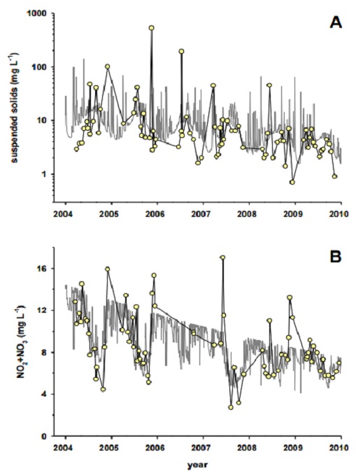
At Blyth Brook (Figure 26A), SS showed a consistent decline from 2004 to 2009. This was evident in both the modelled TWMC as well as in the samples collected from the stream. There was some suggestion, though weaker than for SS, that TP concentrations also followed a similar pattern at Blyth Brook (not shown). Since TP is often sediment-associated, it follows that it too might show a similar trend as SS. This apparent decrease in SS (and possibly TP), over time was not evident in NO2+NO3 or E. coli concentrations at Blyth Brook and was not a general characteristic of the study streams as a group. At Nissouri Creek, both the TWMC and the collected samples for NO2+NO3 showed an apparent decrease in concentration over time (Figure 26B). None of the other measures (E. coli, SS, TP) indicated any trends in this stream.
Since all of the study streams generally experienced the same climatic fluctuations, this cannot explain these apparent trends. While speculative, it is possible that these trends reflect some land use change in the watershed. Detection of early trends such as these might identify streams that warrant further study that is more intensive, since detailed land use and management information would be required to explain such trends. Such work could reveal which land use improvements result in subsequent improvement in water quality. Over time, and with continued monitoring, our ability to discern trends will improve across these study watersheds
Conclusions and future directions
Nutrient concentrations in the study streams were well above pre-impact estimates of these concentrations, with NO2+NO3 concentrations apparently more elevated compared to pre-impact conditions than were TP concentrations. Median TP concentration exceeded the PWQO for TP in 9 of the 15 study streams. For NO3-, median concentrations exceeded the CCME guideline for the protection of aquatic life in 14 of the 15 study streams. As with nutrients,E. coli concentrations in all the study streams were higher than estimates of unimpacted stream concentrations and there was considerable variability among streams.
We observed strong seasonal patterns in nutrient concentrations and loads, with a majority of the annual loads of TP, SS, and NO2+NO3delivered in winter and early spring. The seasonal pattern of E. coli loadings differed from the other measures and was more evenly distributed annually, with autumn showing the highest loading of E. coli to the study watersheds. While seasonal and inter-annual patterns in loading were similar among streams, the magnitude of loads varied substantially among streams, and among parameters within streams. Using coarse-level census data, we found positive relationships between cattle and poultry density with stream nutrient (TP and NO2+NO3) concentrations. Similarly, manure production was positively related with stream nutrient (TP and NO2+NO3) concentrations.
While we found high winter nutrient and SS loads and concentrations, our sampling effort has been quite low during this season, largely because of the logistical challenge in sampling at this time of year. We have increased winter sampling for 2010-2011. This increased winter sampling will improve our load and concentration estimates in the study streams.
Future work, some of which is already underway, will further our understanding of water quality in these streams, and its relationship to land use in their watersheds. One aspect that is currently being examined is the potential impact of the water quality that we observe on the biota of these streams. Stream invertebrates provide an excellent indicator of long-term conditions in streams, their abundance and diversity indicating the suitability of many aspects of the chemical and physical environment for stream biota. Invertebrates have been sampled from these streams for several years, led by the Dorset Environmental Science Centre of the EMRB. These data are currently being analysed and will provide insight into the biotic health of the study streams. Similarly, attached diatoms are indicators of the trophic conditions in streams, acting as temporal integrators of the highly variable nutrient conditions typical of small streams. We have collected diatom samples in 2010 and will repeat collection this season to provide another biotic endpoint to measure stream health.
The potential of agricultural activities to contribute pathogens to source waters is of ongoing interest. One approach to assess this potential is to estimate the load of some pathogens (Cryptosporidium, Campylobacter) from manure using empirical estimates of the number of these pathogens present in various types of manure (Dorner, Huck, & Slawson 2004). This is analogous to the approach we have already used in the present work to estimate nutrient (TP and NO2+NO3) contribution from manure. Thus, in future studies, we will use the manure production data to make similar estimates of the potential contribution of these pathogens from manure in agricultural watersheds in Southwestern Ontario.
The base flow analyses presented here provided some preliminary insight into this aspect of the study streams. As detailed previously, there exists potential in using these base flow data to further our understanding of the nutrient dynamics of these streams, which would aid in guiding management decisions to reduce nutrient concentrations and loads in these streams. For example, some studies have found that a groundwater source having high nitrate concentrations from agricultural inputs resulted in high base flow nitrate concentrations in their study stream (Tesoriero et al. 2009). In such cases, there can be appreciably long recovery times after a reduction in agricultural nitrate inputs, sometimes on the order of decades (Meals, Dressing, and Davenport 2009). Further work assessing the contributions of nitrate from base flow from our streams, and the potential connection to groundwater nitrate would provide an appreciation of the recovery times expected from these systems.
Data from the current study sites provide insight into which watersheds might be worthy of more intensive studies and which sites might be redundant in the nature of the data that they provide. Additional analyses of the existing data will be used to determine the types of watersheds (in terms of land use, stream characteristics, and other attributes) that would be beneficial to add to our suite of study watersheds. Related to this, it is clear that reliable discharge data are critical for load estimation. An evaluation of our study sites in terms of our ability to acquire adequate reliable discharge data is warranted and is currently underway.
While the comparisons with PLUARG revealed several very interesting results, these insights came with several caveats, as our sampling was not specifically created to make these comparisons. The agricultural studies of the PLUARG work were highly labour-intensive and part of a much larger study. A study designed to make comparisons to PLUARG agricultural streams could be tractable if, perhaps, conducted on only a few streams. Additionally, improvements in load estimation, and newer technologies (such as continuous nitrate analysers) could make some aspects of the task less labour-intensive than during the PLUARG study.
Another approach to the examination of land management and its effects on stream water quality is the use of manipulative experiments on small watersheds. Such studies can be designed to be more sensitive to early effects of applying various BMPs on stream water quality. Additionally, the use of control watersheds allows the ability to separate the often-substantial influence of climate, from changes in land management. Our branch is currently involved in an OMAFRA-funded project to study the effects of BMPs on stream water quality. The data we have collected thus far on the 15 watersheds of the present study could provide candidates- perhaps on streams that are typical, or conversely, on ‘outlier’ streams- that would be beneficial for more focussed studies.
As detailed previously, the coarse-scale land use data used in the present work were not ideally suited to the small watersheds that we studied. In spite of this, these data still yielded some suggestive relationships between land use and stream water quality. We are working with OMAFRA to obtain finer scale data on land use practices in the study watersheds. We anticipate that these finer scale data will allow more detailed assessments of how land use and management might be affecting stream water quality. For example, while we were able to approximate manure production in the study watersheds, data that are more detailed will allow the calculation of nutrient mass balances in each watershed. That is, it will allow an accounting of both inputs of nutrients through manure and fertiliser, as well as their removal through export and harvesting of crops. The balance of nutrients in a watershed is likely to relate much more strongly to stream nutrients than is total manure production as we used in the present study. These fine-scale data will also serve to aid in modelling efforts to predict the effects of changing land management, as is currently being done by our branch for Nissouri Creek.
The present monitoring study will provide valuable insight into the effects of changing land use and management practices on the health of these streams, as well as their receiving waters. These changes will take some time to manifest as changes in stream water quality and the present design does not endeavour to control which land use changes and management practices are applied. The study design acts as an ‘observer’ on these changes, which is an invaluable tool in our understanding of how land use and management affect water quality. As Schilling & Spooner (2006) note, without adequate monitoring, improvements through nutrient management efforts may go unappreciated.
References
Alexander, R, R Smith, and G Schwarz. 2000. Effect of stream channel size on the delivery of nitrogen to the Gulf of Mexico. Nature 403, no. 6771 (February): 758-761.
Anon. 1983. Nonpoint Source Pollution Abatement in the Great Lakes Basin An Overview of Post-PLUARG Developments. Report to the Great Lakes Water Quality Board, Windsor, Ontario.
Anon. 2009. Guidelines for Canadian Recreational Water Quality, Third Edition. Document for Public Comment. Health Canada.
Caraco, N.F., J.J. Cole, G.E. Likens, G.M. Lovett, and K.C. Weathers. 2003. Variation in NO3- Export from Flowing Waters of Vastly Different Sizes: Does One Model Fit All? Ecosystems 6, no. 4 (June): 344-352.
Carpenter, S.R., N.F. Caraco, D.L. Correll, R.W. Howarth, N. Sharpley, and V. H. Smith. 1998. Nonpoint Pollution of Surface Waters With Phosphorus and Nitrogen. Ecological Applications 8, no. 3 (August): 559-568.
Chambers, P.A., M. Guy, S.S. Dixit, G.A. Benoy, R.B. Brua, J.M. Culp, D. McGoldrick, B.L. Upsdell, and C. Vis. 2009. Nitrogen and Phosphorus Standards to Protect the Ecological Condition of Canadian Streams, Rivers and Coastal Waters. National Agri-Environmental Standards Initiative Synthesis report No. 11. Environment Canada. Gatineau, Quebec.
Chang, H., B.M. Evans, and D.R. Easterling. 2001. The effects of climate change on stream flow and nutrient loading. Journal of the American Water Resources Association 37, no. 4 (August): 973-985.
Chesters, G., J. Robinson, R. Stiefel, R. Ostry, T. Bahr, RD Coote, and D. M Whitt. 1978. Pilot Watershed Studies Summary Report. Ontario Ministry of the Environment.
Clerk, S. 2007. Nutrient Management Monitoring Program: 2005 Annual Technical Report (May). Ontario Ministry of the Environment.
Coote, D, and R DeHaan. 1978. Agricultural Watersheds Overview Data Analysis And Extrapolation Final Report - Project 1B Agricultural Watershed Studies Task Group C (Canadian Section) Activity 1 , International Reference Group On Great Lakes Pollution From Land Use Activities.
Dinnes, D.L. D.L. Karlen, D.B. Jaynes, and T.C. Kaspar. 2002. Nitrogen management strategies to reduce nitrate leaching in tile- drained Midwestern soils. Agronomy Journal 94: 153-171.
Donnison, A., C. Ross, and B. Thorrold. 2004. Impact of land use on the faecal microbial quality of hill-country streams. New Zealand Journal of Marine and Freshwater Research 38, no. 5 (December): 845-855.
Dorner, S.M, P.M. Huck, and R.M. Slawson. 2004. Estimating potential environmental loadings of Cryptosporidium spp. and Campylobacter spp. from livestock in the Grand River Watershed, Ontario, Canada. Environmental Science & Technology 38, no. 12 (June): 3370-3380.
Eckhardt, K. 2008. A comparison of baseflow indices, which were calculated with seven different baseflow separation methods. Journal of Hydrology, 352 (1-2), 168-173.
Edge, T.A., I. Droppo, A. El-Shaarawi, V. Gannon, M. Hewitt, R. Kent, I. Khan, et al. 2009. An Evaluation of Escherichia coli as a Potential Agri-Environmental Waterborne Pathogen Standard. Synthesis Report No. 14. National Agri-Environmental Standards Initiative. Environment Canada. Gatineau, Quebec.
Environmental Commissioner of Ontario. 2004. "The Nutrient Management Regulation." Choosing our Legacy, ECO Annual Report, 2003-04. Management. Toronto: The Queen’s Printer for Ontario. 74-78.
Environmental Commissioner of Ontario. 2006. "Amending the Nutrient Management Regulation." Neglecting our Obligations, ECO Annual Report, 2005-06. Management. Toronto: The Queen’s Printer for Ontario. 111-116.
Gburek, W.J., and A.N. Sharpley. 1998. Hydrologic Controls on Phosphorus Loss from Upland Agricultural Watersheds. Journal of Environmental Quality 27: 267-277.
Gordon, N.D. 2004. Stream Hydrology: An Introduction For Ecologists. John Wiley and Sons.
Graves, A.K., Hagedorn, C., Brooks, A., Hagedorn, R.L., and Martin, E. 2007. Microbial source tracking in a rural watershed dominated by cattle. Water Res. 41: 3729–3739.
Green, M.B., J.L. Nieber, G. Johnson, J. Magner, and B. Schaefer. 2007. Flow path influence on an N:P ratio in two headwater streams: A paired watershed study. Journal of Geophysical Research 112, no. G3 (September): 1-11.
Gustafson, A., S. Fleischer, and A. Joelsson. 2000. A catchment-oriented and cost-effective policy for water protection. Ecological Engineering 14, no. 4 (April): 419-427.
Hoffman, M, and H. Johnsson. 2000. Nitrogen in Sweden Leaching from Agricultural Land Model Calculated Effects of Measures to Reduce Leaching Loads. Ambio 29, no. 2: 67-73.
Hoffman, N, and M.S. Beaulieu. 2006. A Geographical Profile of Manure Production in Canada, 2001. Minister of Industry. Ottawa, Ontario, Canada.
Hunter, C, and A. McDonald. 1991. Seasonal changes in the sanitary bacterial quality of water draining a small upland catchment in the Yorkshire dales. Water Research 25, no. 4 (April): 447-453.
Hunter, C., J. Perkins, J. Tranter, and J. Gunn. 1999. Agricultural land-use effects on the indicator bacterial quality of an upland stream in the Derbyshire peak district in the U.K. Water Research 33, no. 17 (December): 3577-3586.
Jamieson, T.S. 2010. Quantification of Oxygen Dynamics in the Grand River Using a Stable Isotope Approach. PhD thesis. University of Waterloo. Waterloo, Ontario, Canada.
Jensen, F. 2003. Nitrite disrupts multiple physiological functions in aquatic animals. Comparative Biochemistry and Physiology - Part A: Molecular & Integrative Physiology 135, no. 1 (May): 9-24.
Kon, T., Weir, S. C., Howell, E. T., Lee, H., & Trevors, J. T. 2009. Repetitive element (REP) - polymerase chain reaction (PCR) analysis of Escherichia coli isolates from recreational waters of Southeastern Lake Huron. Canadian Journal of Microbiology, 55: 269-276.
Kowalenko, C.G. 1978. Nitrogen transformation processes in agricultural watershed soils final report on Project 11 Agricultural Watershed Studies. International Reference Group on Great Lakes. Pollution from Land Use Activities. International Joint Commission.
Lewis, T.W., and J.C. Makarewicz. 2009. Winter application of manure on an agricultural watershed and its impact on downstream nutrient fluxes. Journal of Great Lakes Research 35: 43-49.
Lewis, W. and D.P. Morris. 1986. Toxicity of nitrite to fish: A Review. Transactions of the American Fisheries Society 115: 183-195.
Lim, K.J., B.A. Engel, Z. Tang, J. Choi, K. Kim, S. Muthukrishnan, and D. Tripathy. 2005. Automated web GIS based hydrograph analysis tool, WHAT. Journal of the American Water Resources Association 41, no. 6 (December): 1407-1416.
Logan, T.J. 1982. Mechanisms for release of sediment-bound phosphate to water and the effects of agricultural land management on fluvial transport of particulate and dissolved phosphate. Hydrobiologia 91-92, no. 1 (July): 519-530.
Maguire, R.O., G.H. Rubaek, B.E. Haggard, and B.H. Foy. 2005. Critical evaluation of the implementation of mitigation options for phosphorus from field to catchment scales. Journal of Environmental Quality 38, no. 5: 1989-1997.
McDowell, R.W., B.J.F. Biggs, A.N. Sharpley, and L. Nguyen. 2004. Connecting phosphorus loss from agricultural landscapes to surface water quality. Chemistry in Ecology 20, no. 1: 1-40.
Meals, D.W., S.A. Dressing, and T.E. Davenport. 2009. Lag time in water quality response to best management practices: a review. Journal of Environmental Quality 39, no. 1: 85-96.
Mohamed, M., T. Howell, and A. Todd. 2009. Water Quality on the Shores of Lake Huron Adjacent to the Saugeen, Maitland, and Bayfield River Mouths. Ontario Ministry of the Environment, Environmental Monitoring and Reporting Branch.
Moog, D.B, and P.J. Whiting. 2002. Climatic and agricultural contributions to changing loads in two watersheds in Ohio. Journal of Environmental Quality 31, no. 1: 83-89.
Moran, E.C., and D.O. Woods. 2009. Comprehensive watershed planning in New York State: The Conesus Lake example. Journal of Great Lakes Research 35: 10-14.
Nangia, V., D. J. Mulla, and P.H. Gowda. 2010. Precipitation changes impact stream discharge, nitrate–nitrogen load more than agricultural management changes. Journal of Environmental Quality 39, no. 6: 1-9.
Neilsen, G.H., J.L. Culley, and D.R. Cameron. 1978. Nitrogen Loadings From Agricultural Activities In The Great Lakes Basin Integration Report On Nitrogen. International Reference Group on Great Lakes Pollution from Land Use Activities. International Joint Commission.
O'Rourke, N. Hatcher, L. and Stepanski, E. 2005. A Step-by-Step Approach to Using SAS for Univariate and Multivariate Statistics, Second Edition. SAS Press and John Wiley Sons Inc.
Ongley, E.D. 1978. Land use, Water Quality and River-Mouth Loadings : a Selective Overview for Southern Ontario by International Reference Group on Great Lakes Pollution from Land Use Activities. International Joint Commission.
Ontario Ministry of Environment and Energy. 1994. Water Management policies and guidelines, Provincial Water Quality Objectives. PIBS 3303E. Queen’s Printer for Ontario.
Quinn, G.P. and Keough, M.J. 2002. Experimental Design and Data Analysis for Biologists. Cambridge University Press. Cambridge, U.K.
Rantz, S.E. 1982. Measurement of Streamflow : Volume 1. Measurement and Discharge and Computation Volume of Stage. Geological Survey Water-Supply Paper 2175. United States Geological Survey. United States Government Printing Office, Washington, USA.
Rosamond, M.S., S.J. Thuss, S.L. Schiff, and R.J. Elgood. 2011. Coupled cycles of dissolved oxygen and nitrous oxide in rivers along a trophic gradient in southern Ontario, Canada. Journal of Environmental Quality 40, no. 1: 256-270.
Runkel, R.L, C.G. Crawford, and T.A. Cohn. 2004. Load Estimator (Loadest ): A Fortran Program For Estimating Constituent Loads In Streams And Rivers Techniques And Methods Book 4, Chapter A5 A FORTRAN Program for Estimating Constituent Loads in Streams and Rivers. Reston, Virginia.
Sanchez, C.A., and A.M. Blackmer. 1988. Recovery of anhydrous ammonia-derived nitrogen-15 during three years of corn production in Iowa. Agronomy Journal 80, no. 1: 102-108.
Sandstedt, C.A. 1990. Nitrates: sources and their effects upon humans and livestock. American University. Washington, D.C.
Schelde, K., L.W. de Jonge, C. Kjaergaard, M. Laegdsmand, and G.H. Rubæk. 2006. Effects of Manure Application and Plowing on Transport of Colloids and Phosphorus to Tile Drains. Vadose Zone Journal 5, no. 1 (March): 445-458.
Schilling, K.E., and J. Spooner. 2006. Effects of watershed-scale land use change on stream nitrate concentrations. Journal of Environmental Quality 35, no. 6: 2132-2145.
Schilling, K.E., and Y. Zhang. 2004. Base flow contribution to nitrate-nitrogen export from a large, agricultural watershed, USA. Journal of Hydrology 295, no. 1-4 (August): 305-316.
Sklash, M. G., Gillham, R. W., & Cherry, J. A. 1978. Studies Of The Agricultural Contribution To Nitrate Enrichment Of Groundwater And The Subsequent Nitrate Loading. Part III: Mechanisms Of Runoff Generation And Nitrate Flux To Streams During Runoff Events. Final report Project No. 41122 A PLUARG, Task Group C Study.
Smith, R.A., R.B. Alexander, and G.E. Schwarz. 2003. Natural background concentrations of nutrients in streams and rivers of the conterminous United States. Environmental Science & Technology 37, no. 14 (July): 3039-3047.
Smith, V.H. 2003. Eutrophication of freshwater and coastal marine ecosystems: a global problem. Environmental Science and Pollution Research International 10, no. 2 (January): 126-39.
Soil Resource Group. 2010. Agricultural land management and water quality data evaluation in representative agricultural watersheds in the Grand River and Thames River basins. OMAFRA Great Lakes Project 07-054.
Stewart, W.M., D.W. Dibb, A.E. Johnston, and T.J. Smyth. 2005. The Contribution of Commercial Fertilizer Nutrients to Food Production. Agronomy Journal 97, no. 1: 1-7.
Tesoriero, A.J., J.H. Duff, D.M Wolock, N.E Spahr, and J.E. Almendinger. 2009. Identifying pathways and processes affecting nitrate and orthophosphate inputs to streams in agricultural watersheds. Journal of Environmental Quality 38, no. 5: 1892-1900.
Todd, A. 2006. Water Sample Collection and Submission Protocols for Partners in the Provincial Water Quality Monitoring Network.
Vitousek, P.M, J.D. Aber, R.W. Howarth, G.E. Likens, P.A. Matson, D.W. Schindler, W.H. Schlesinger, and D.G. Tilman. 1997. Human alteration of the global nitrogen cycle: sources and consequences. Ecological Applications 7, no. 3: 737-750.
Zuur, A.F., Ieno, E.N., and Smith, G.M. 2007. Analysing ecological data. Springer Science + Business Media. New York.
Appendix - Detailed Maps of the Study Watersheds
Figure A-1: Avon River watershed.
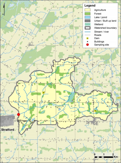
Figure A-2: Blyth Brook watershed. Legend as in Figure A-1.
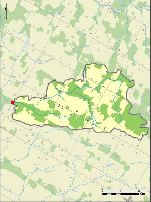
Figure A-3: Falkland Creek watershed. Legend as in Figure A-1.
Figure A-4: Griffins Creek watershed. Legend as in Figure A-1.
Figure A-5: The Little Ausable River watershed. Legend as in Figure A-1.
Figure A-6: Middle Maitland watershed. Legend as in Figure A-1.
Figure A-7: Muskrat Creek watershed. Legend as in Figure A-1.
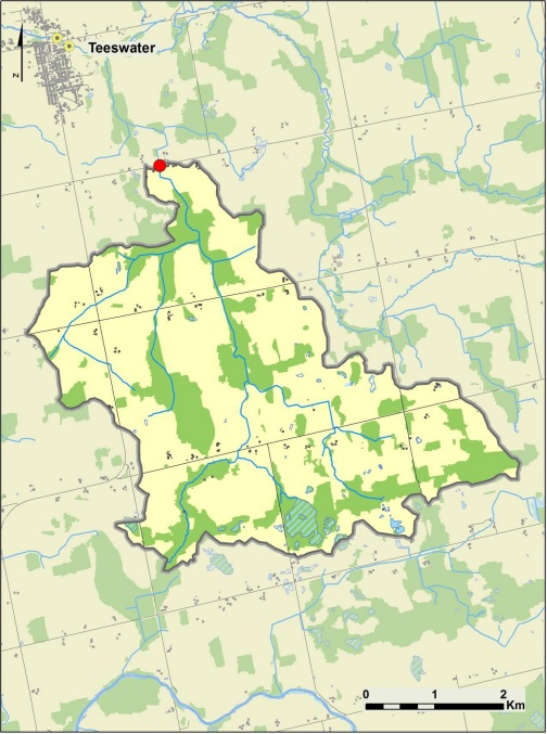
Figure A-8: Nineteen Creek watershed. Legend as in Figure A-1.
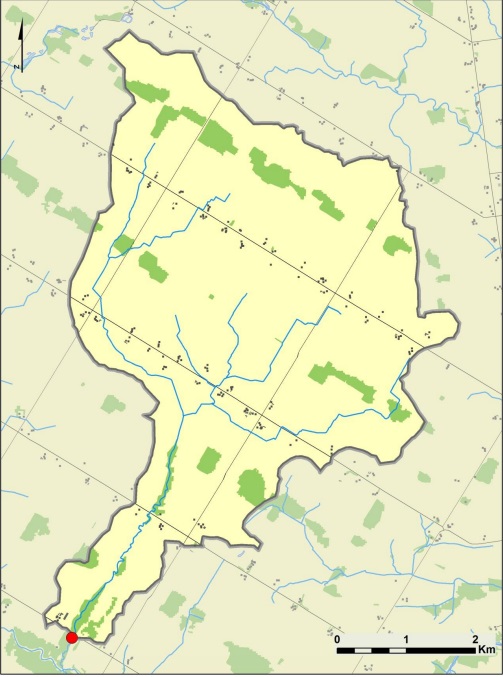
Figure A-9:Nissouri Creek watershed. Legend as in Figure A-1.
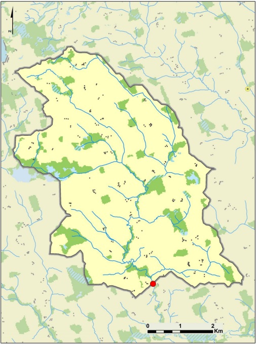
Figure A-10: The South Thames River watershed. Legend as in Figure A-1.
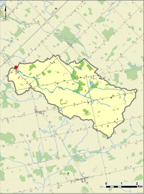
Figure A-11: Salem Creek watershed. Legend as in Figure A-1.
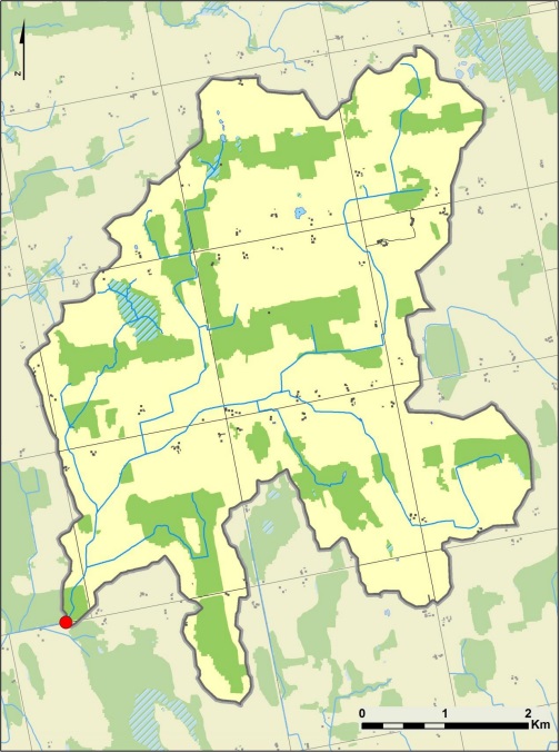
Figure A-12: Silver Creek watershed. Legend as in Figure A-1.
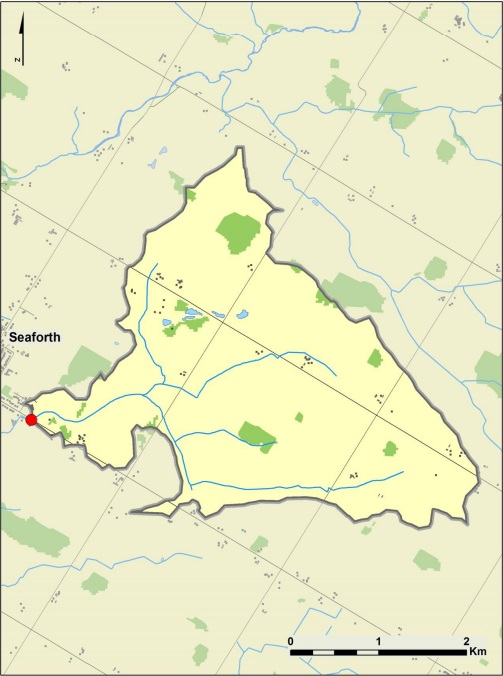
Figure A-13: Stirton Creek watershed. Legend as in Figure A-1.
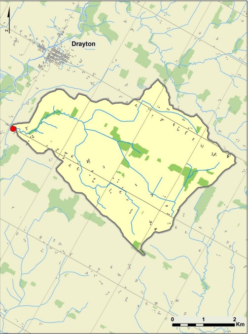
Figure A-14: Thames River watershed. Legend as in Figure A-1.
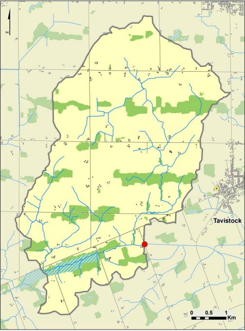
Figure A-15: Trout Creek watershed. Legend as in Figure A-1.
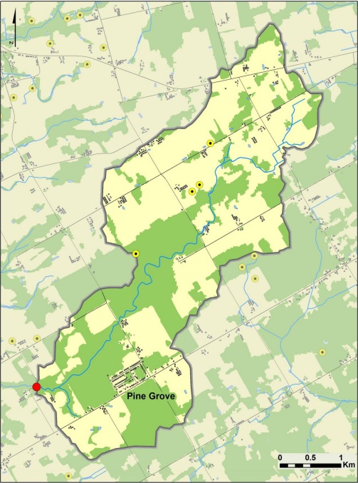
Footnotes
- footnote[1] Back to paragraph Location refers to sampling site at watershed outlet
- footnote[3] Back to paragraph Ontario Land Cover Database (1999)
- footnote[2] Back to paragraph Per cent of farms with a Nutrient Management Plan, Data from OMAFRA, 2005
- footnote[*] Back to paragraph could not be determined due to data suppression (see text)
- footnote[a] Back to paragraph Detection limit = 0.025 µg N L-1
- footnote[b] Back to paragraph Detection limit = 4 CFU 100 mL-1