Methodology to define the Built Boundary for the Greater Golden Horseshoe

SECTION 2.  Methodology to Define the Built Boundary for the Greater Golden Horseshoe

The methodology, the Ministry of Public Infrastructure Renewal has used to define the built boundary, has four steps. The first three steps involve a GIS analysis of the primary data to determine the approximate extent of built-up areas in the Greater Golden Horseshoe. Step 4 involves verification and refinement of the built boundary.

Step 1: Create a Parcel Land-Use Database

Step 1 involves the selection and compilation of the primary data sources.

1.1 Select the most appropriate primary datasets

The first step in developing the built boundary is the selection of appropriate primary data sources, which can be used to identify urbanized areas. A number of basic criteria are used in order to select appropriate datasets. The data needs to be:

• consistently available and applicable across the entire Greater Golden Horseshoe;
• able to identify land use on a consistent, Greater Golden Horseshoe-wide geography to determine built-up uses;
• compatible with local and regional planning practices, and land-use and planning boundaries;
• able to maintain privacy of confidential, property-related information; and
• able to track the location and amount of new residential units annually over the life of the Growth Plan.

The scale of the geographic unit of the primary datasets is also a critical factor since it determines the precision and character of the built boundary. The unit of geography used in the analysis, in this case the property parcel, is the building block for the built boundary line.

The primary datasets that meet the criteria above are:

1. Tax Roll 2006 MPAC data (current to end of 2005) 
   MPAC administers a uniform, province-wide property assessment system, including a database of property types using registered Land Transfer Tax Affidavits. MPAC data is classified into property types or land uses such as commercial, industrial, residential, farm, multi-residential, and vacant. (Note: Rule vii in Step 4 allows for including built-up parcels that are not captured in the MPAC dataset but that were built-up as of June 16, 2006.)
2. OPA data (current to May 2006) 
   OPA is jointly maintained by Teranet Enterprises Inc., MPAC and the Ministry of Natural Resources. It contains a standardized, Ontario-wide, geospatial dataset of assessment, ownership and Crown parcels of land. The OPA database includes parcel boundaries, assessment roll numbers, and property identification numbers where applicable.

It is important to note that the OPA and MPAC datasets obtained by the Ministry of Public Infrastructure Renewal contain only land-use, residential unit-count, and parcel number information. The datasets used to develop this methodology, and applied in this analysis, do not contain any confidential, personal or financial information.

For a detailed description of these two datasets and a list of attributes contained in the MPAC dataset obtained by the Ministry of Public Infrastructure Renewal, please refer to Appendices 2 and 3 of this paper.

Other datasets that were evaluated by the Ministry of Public Infrastructure Renewal for their suitability are also listed and described in more detail in Appendix 4.

1.2 Summarize land use data into manageable categories for further analysis

The MPAC dataset contains approximately 300 land-use attribute codes. This is more detail than is required for this analysis. These 300 codes are therefore sub-divided into six broader, simplified summary land uses: built, unbuilt, green space unavailable, variable, not a parcel, and unknown. These six summary uses are further reclassified into only built and unbuilt later in Step 3.

Please see Appendix 3 for a full list of detailed MPAC land-use codes and their corresponding summary land-use coding.

1.3 Compile the database using primary datasets

The next step is to create an integrated database by linking the parcel number attributes in the two selected datasets in order to combine parcel boundary, residential unit count and land-use information. This combined parcel and land-use database is then used to determine which OPA parcels are considered built or unbuilt.

MPAC data and OPA datasets are linked to create a database with one record per parcel^{footnote 1[1]}. Each parcel's land use, geographic boundaries, and residential unit attributes are identified. Figure 4 illustrates the linking process for these two datasets.

Where records with multiple MPAC land-use codes are assigned to a single parcel (e.g. one parcel can contain both residential and recreational land uses), the parcel is classified as built, provided that at least one of the land-use codes assigned to the parcel has a known built use (e.g. residential). A parcel with multiple MPAC land-use codes is classified as unbuilt if all the property codes associated with it are unbuilt land uses.

Condominium files are aggregated to create parcel level data and not residential unit level data. The unique roll number allows for identification of which units corresponded to a particular condominium parcel. A separate joining process for condominiums and their associated units is carried out to assign the unit data to its respective parcel.

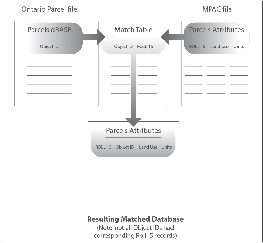
Figure 4: Linking MPAC and OPA datasets

The number of residential units on each parcel is computed and recorded. This allows for the calculation in Step 2 of the number of residential units in settlement areas. It also allows for the development of a baseline count for the number of residential units within the final built boundary, and will assist with tracking new residential units to assess achievement of the Growth Plan's intensification policies.

Step 2: Select Settlement Areas for which a Built Boundary will be Developed

In Step 2, settlement areas containing over 400 residential units are identified. By definition, the built-up area and built boundary must lie within a settlement area. The Growth Plan aims to direct intensification to settlement areas that can accommodate and service new growth. However, some settlement areas identified in local official plans are small, not fully serviced, and may not be appropriate as a focus for intensification.

The 400-unit threshold corresponds approximately with settlement areas that have full municipal servicing and capacity to support intensification and future growth.

2.1 Compile settlement area dataset

The Ministry of Municipal Affairs and Housing maintains land-use data derived from the latest, approved, publicly available individual municipal official plans. This information is used to compile a dataset of lands in the Greater Golden Horseshoe that are considered settlement areas as defined in the Growth Plan^{footnote 2[2]}. These lands are designated in the respective official plans for development and urban uses. The built boundary is developed for settlement areas identified as such in approved upper- and single-tier official plans. The approved lower-tier official plan is used where no upper-tier official plan exists.

2.2 Establish threshold size and identify settlement areas for which a built boundary will be developed

The Ministry of Public Infrastructure Renewal determined that the built boundary would be developed for settlement areas over a size threshold of 400 residential units. The cut-off of 400 residential units translates to approximately 1,000 persons based on an average household size of approximately 2.5 persons per residential unit^{footnote 3[3]} in the Greater Golden Horseshoe. This is consistent with Statistics Canada's cut-off of 1,000 persons for its definition of an urban area based on international comparative research.

In Step 4, all settlement areas of all sizes are reviewed again in consultation with their respective municipalities for suitability to accommodate intensification before a built boundary is delineated. Some settlement areas and their corresponding grid cells which are dropped in this step may be included again in Step 4.

Using the parcel land-use database, a count of residential units is run for all parcels contained within each polygon in the settlement area dataset. A parcel is counted inside of the settlement area if its geometric centre lies within the settlement area boundary. Individual settlement areas polygons (e.g. individual towns, hamlets, etc.) are treated separately in this analysis.

Polygons with 400 or more residential units are then selected.

Figure 5 illustrates the application of this threshold to the settlement area dataset. The red polygons on the map represent settlement areas containing fewer than 400 residential units. The pink areas represent settlement areas containing 400 or more residential units which met the threshold and are selected in this step. All settlement areas in the dataset containing fewer than 400 residential units are excluded.

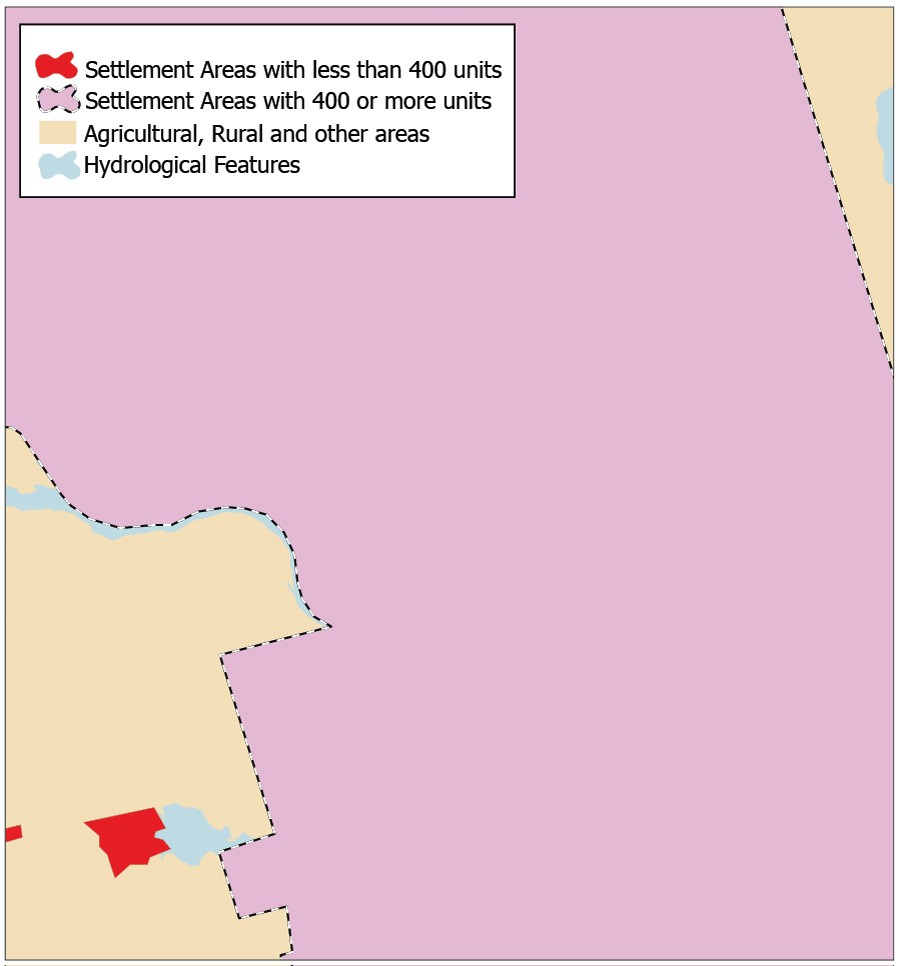
Figure 5: Identification of threshold settlement areas for which a built boundary will be developed.

Step 3: Generate Grid-cell Mapping for the Settlement Areas Identified in Step 2

This third step uses the MPAC-OPA database compiled in Step 1 and the settlement areas greater than the threshold size selected in Step 2, to identify and aggregate the land use information in the parcel and land-use database using a grid-cell overlay in order to manage the millions of parcel and land-use records.

3.1 Overlay grid-cell matrix on Growth Plan area

A grid-cell matrix is overlaid and used as a base to manage, group, and aggregate millions of land use and parcel records, making them standardized and manageable for further analysis. The grid-cell matrix is comprised of 250m X 250m square cells overlaid across the entire Greater Golden Horseshoe^{footnote 4[4]}.

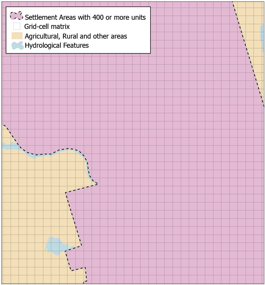
Figure 6: Overlay of grid-cell matrix.

The approximately 545,000 grid-cells covering the geography of the Greater Golden Horseshoe allow for the grouping of underlying land-use and parcel codes into each corresponding cell while still being small enough to accurately represent the underlying land use^{footnote 5[5]}. Using a larger grid cell reduces the accuracy of the methodology. A smaller grid cell increases the computational challenges without any real improvement in the accuracy of the methodology.

Figure 6 illustrates the overlay of the grid-cell matrix on the settlement area base created in Step 2.

3.2 Assign one of six summary land uses to each grid cell in the Growth Plan area

Summary land uses identified in Step 1.3 are assigned to grid cells for the purpose of aggregation and further generalization. This step establishes whether a cell has enough of a particular summary land use in it to represent that use.

The land area of each summary land use in each cell is computed. The cell is given the summary land use that had the highest percentage of land area within that cell.

Figure 7 illustrates how the dominant summary land use of several parcels contained within an individual grid cell is assigned to that particular grid cell.

Each grid cell is given one of the six summary uses developed in Step 1.2. Figure 8 illustrates the assignment of dominant land uses to the grid-cell matrix.

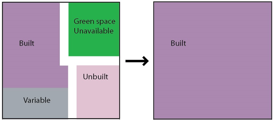
Figure 7: Assignment of dominant summary land use to a grid cell.

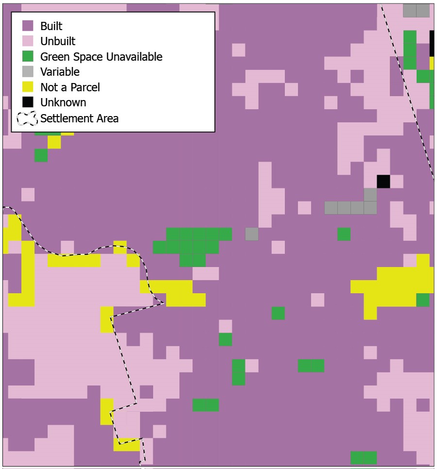
Figure 8: Assignment of dominant land uses to the grid-cell matrix.

3.3 Select all cells that fall within settlement areas over the threshold size

This step determines which grid cells fall within the selected settlement areas for which a built boundary will be developed. Grid cells and their corresponding summary land uses qualify as belonging to a settlement area if 50 per cent or more of the cell's area lies within the settlement area boundary.

All cells that fall outside the threshold settlement areas, though identified as built in Step 3.2, are dropped from the database and not included in the next steps of the methodology as they lie in settlement areas that have fewer than 400 residential units or lie outside of settlement area boundaries.

However, as mentioned above, in Step 4, all settlement areas of all sizes are reviewed again in consultation with their respective municipalities for suitability to accommodate intensification before a built boundary is delineated. Some settlement areas and their corresponding grid cells which are dropped in this step may be included again in Step 4.

Figure 9 illustrates the selection of grid cells that fall within settlement areas for which a built boundary will be developed.

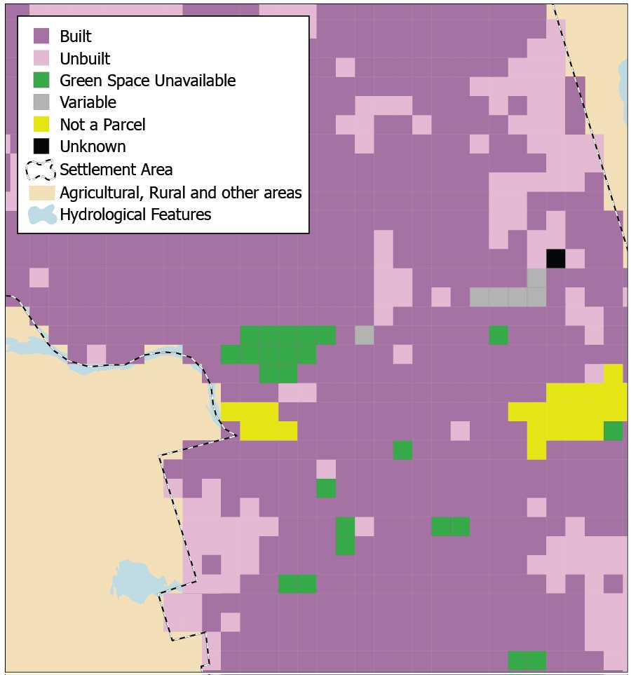
Figure 9: Selection of cells that fall within settlement areas for which a built boundary will be developed.

3.4 Assign all grid cells as either built or unbuilt

In this step, summary land uses are further reclassified as either built or unbuilt based on their land-use attributes. Cells coded as variable, no parcel, and greenspace not available, are all converted to built grid cells. All unknown cells are converted to unbuilt.

This is done to create two broad categories and to identify only those cells that represented built-up areas on the ground, prior to their further generalization and aggregation in Step 3.5.

Figure 10 illustrates the result of the conversion of the six summary land uses given to cells (illustrated in Figure 9), to the two categories of built and unbuilt.

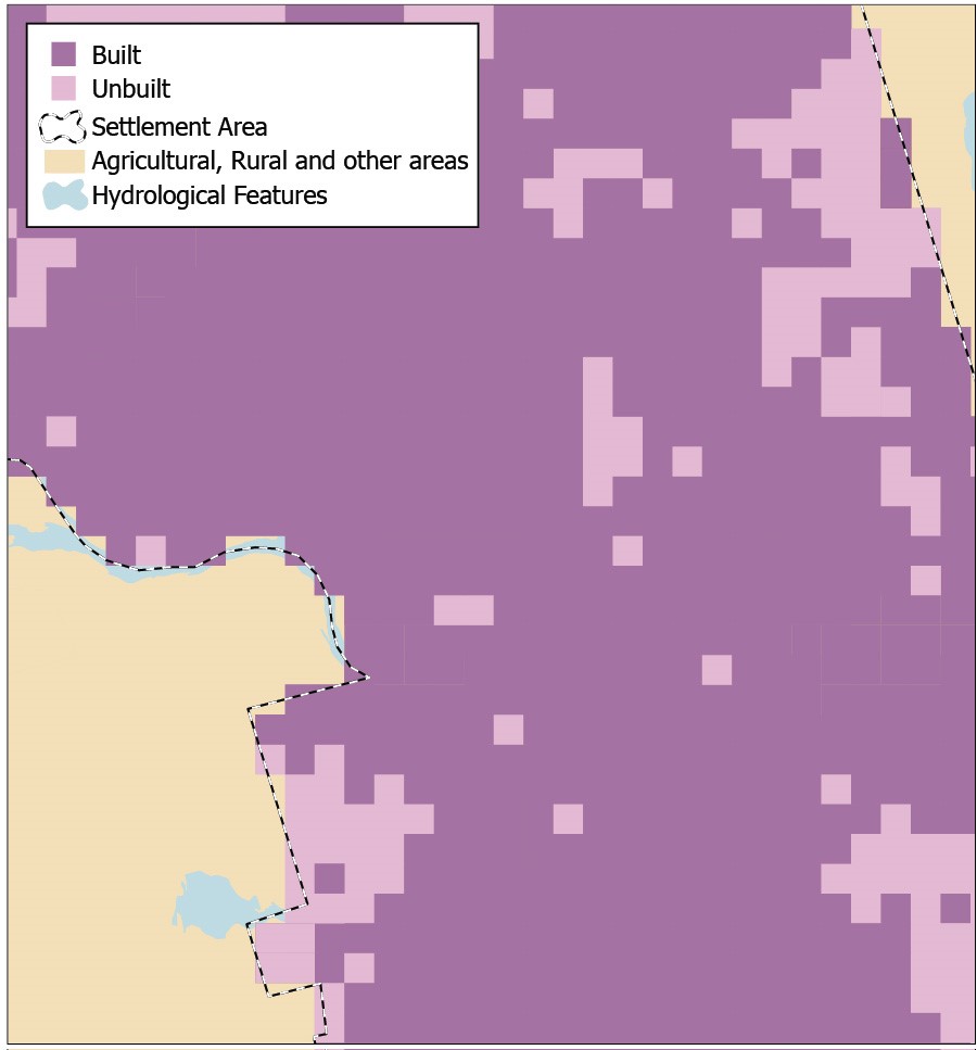
Figure 10: Assignment of six summary land uses to the two categories of built and unbuilt.

3.5 Consolidate and aggregate the built grid cells to approximately identify built-up areas

The result of Step 3.4 includes built grid-cells in large, contiguous groupings that represent established built-up areas on the ground, or cells scattered on the periphery that represent newer, non-contiguous, fringe development.

Step 3.5 uses automated GIS operations applied in sequence to consolidate built grid-cells representing established built-up areas. This step also links smaller groupings of built grid cells, usually representative of patchwork development on the fringe of urban areas which are in the process of being developed, to larger groupings of built grid cells to make them contiguous. This step also drops built grid cells that are scattered or non-contiguous.

The following GIS operations constitute this step:

1. Join nearby cells or groups of cells: 
   If a built grid cell or group of built grid cells are separated by only one cell width from another built grid cell or group of built grid cells, the one-cell width of unbuilt grid cell is reassigned as built^{footnote 6[6]}. Built grid cells touching on their diagonals are considered to be contiguous and joined to their adjacent cells. The grid cells reassigned from unbuilt to built are illustrated in Figure 11. This step is intended to include fringe development that is developed enough and close to larger, established built-up areas to be considered contiguous with them.
    

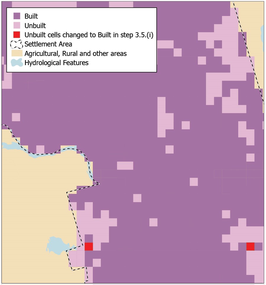
Figure 11: Application of step 3.5.(i) – Joining nearby cells or groups of cells.

2. Drop cells or small groups of cells that are further away and on their own: 
   On completion of Step 3.5.(i) above, separate groupings of fewer than eight contiguous built grid cells, containing fewer than 400 residential units, are reclassified as unbuilt grid cells so as to exclude stand-alone built-up areas that are too small to contribute meaningfully to the intensification objectives of the Growth Plan. Figure 12 illustrates this step. 
    

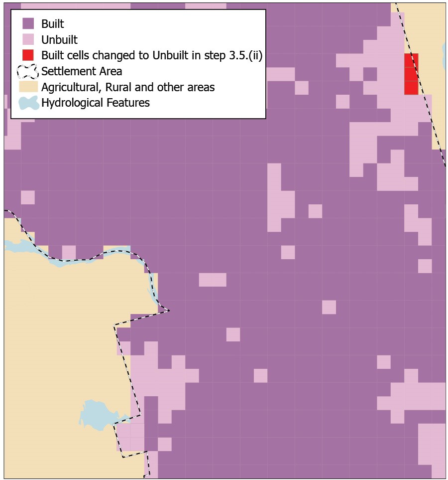
Figure 12: Application of step 3.5.(ii) – Dropping cells or small groups of cells that are further away and on their own.

3. Fill in small groups of unbuilt cells that are surrounded by built cells: 
   On completion of Step 3.5.(ii) above, groupings of fewer than six contiguous unbuilt grid cells that are surrounded by built grid cells, are reclassified as built. This results in a more contiguous built area. Any future development within the small areas added in this step would be supportive of the Growth Plan's intensification objectives. Or, these areas may represent small parks and open areas, the uses of which would remain unchanged if included in the built boundary. Figure 13 illustrates this step. 
    

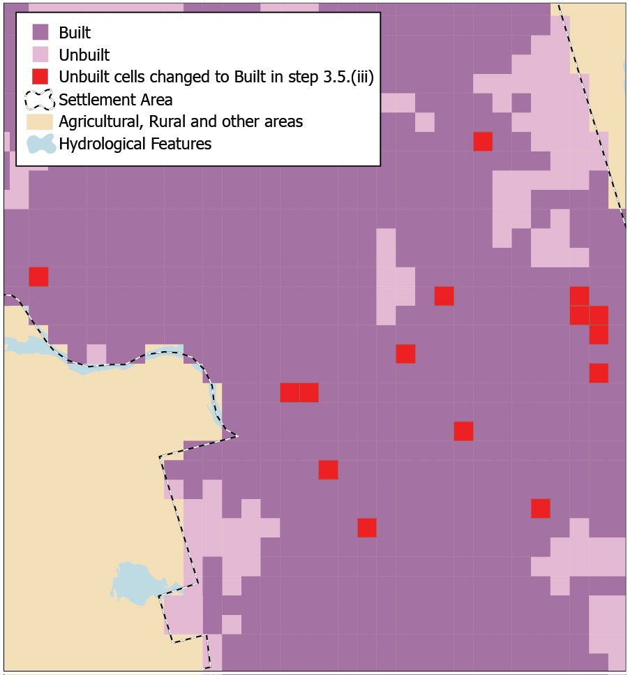
Figure 13: Application of step 3.5.(iii) - Filling in small groups of unbuilt cells that are surrounded by built cells.

Step 4: Refine the Grid-cell Mapping to Create a Built Boundary

Step 4 involves verification and refinement of the grid-cell mapping to create a detailed built boundary that can be identified on the ground. This step provides a final set of refinement rules to apply to the grid-cell mapping, using a variety of GIS and other data sources such as MPAC and OPA data, orthophotography, building starts and completions, official plan schedules, road networks, and water features to delineate a built boundary that is identifiable on the ground and aligned with roads, water features, and property parcels.

The Ministry of Public Infrastructure Renewal has worked in consultation with single-, upper- and lower-tier municipalities, as well as stakeholders and other public bodies, to apply these final refinement rules in a consistent manner across the Greater Golden Horseshoe.

The following refinement rules are applied in sequence to the built grid cells generated in Step 3 to create a built boundary for the Greater Golden Horseshoe.

Rule i. Refine settlement areas for which a built boundary will be delineated

In Rule i, all settlement areas, including those identified in Step 2 are further reviewed for suitability to accommodate intensification, prior to delineating a built boundary.

A precise boundary is delineated for those settlement areas, identified in consultation with municipalities, that have full municipal services, will be a focus for intensification, or will accommodate significant future growth.

Undelineated built-up areas for smaller, unserviced or partially-serviced settlement areas, which have limited capacity to accommodate significant future growth, are represented as dots in the maps in Section 3. These settlement areas are typically small towns and hamlets. Since they are not expected to be a focus for intensification, they do not require a delineated built boundary for future monitoring purposes.

The built boundary is developed for settlement areas identified as such in approved upper- and single-tier official plans. The approved lower-tier official plan is used where no upper-tier official plan exists.

Where two settlement areas are adjacent, functionally connected, and within the same upper- or single-tier municipality, they are considered a single settlement area for the purposes of delineating a built boundary.

Rule ii. Revert from grid cells to parcels

The grid-cell mapping in Step 3 provides for a coarse identification of built-up areas, and does not follow parcel or road boundaries. In Rule ii, the parcel boundaries are overlaid on the grid cell map and each parcel is categorized as either built or unbuilt. Parcels whose geometric centres fall within built or unbuilt grid cells are assigned that corresponding built or unbuilt status. The grid-cell structure is then removed, leaving only the OPA parcel fabric with its built and unbuilt attributes as a starting point for further refinement. The outcome of this rule is illustrated in Figure 14.

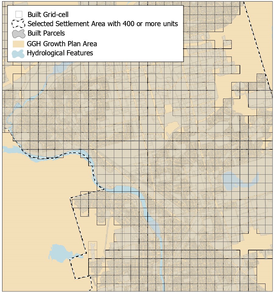
Figure 14: Illustration of built parcels falling within built grid cells.

Rule iii. Verify land uses of parcels

In this refinement rule, parcels assigned as built but which are known through more detailed local knowledge or data to be unbuilt, are reassigned as unbuilt. MPAC data may have several land uses for a single parcel which results in parcels with predominantly non-urban, unbuilt uses on them appearing as built. Also, some gravel pits, golf courses, campgrounds, private parks, etc. are re-classified as unbuilt if they are considered interim uses by the respective municipality.

Rule iv. Assign all brownfield sites and greyfield sites as built

Brownfield sites or greyfield sites not already identified as built in previous steps are identified through consultation with municipalities and classified as built.

Rule v. Reassign certain unbuilt parcels adjacent to Provincial 400-series highways as built

Unbuilt parcels lying between the built parcel edge and the centre-line of a 400-series provincial highway are reassigned as built, when the distance between the outer edge of the nearest built parcel and the centre-line of the highway is less than 1km. Otherwise they are treated as unbuilt.

Figures 15a and 15b below illustrate the application of this refinement rule.

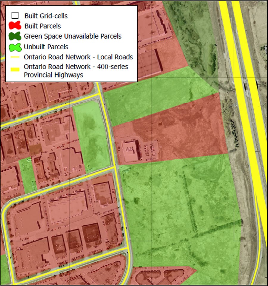
Figure 15a

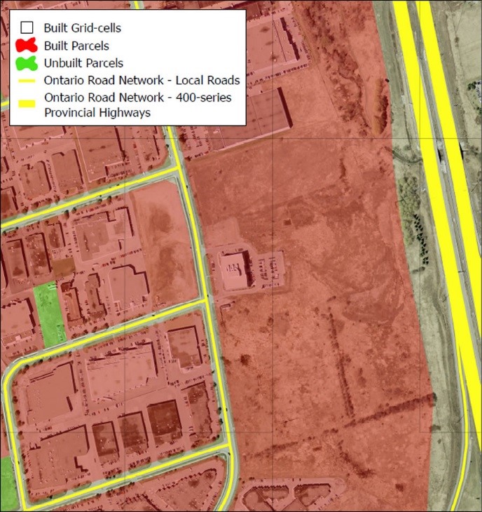
Figure 15b

Rule vi. Include land uses that are in their final form within the built boundary

Parcels currently occupied by the features or uses listed below are considered built since they are in their final form i.e. not available for redevelopment, and when they are surrounded by or adjacent to built parcels.

• Municipal, federal and provincial parks.
• Existing servicing and community infrastructure such as water and sewage treatment plants, landfills, water towers, cemeteries, school yards, etc.
• Transportation infrastructure such as highway rights-of-way, highway interchanges, canals, airports, rail yards, active railway rights-of-way, docks etc.

Natural heritage features and areas, and floodplains where development is expressly prohibited, and which are completely surrounded by built parcels are also included in the built boundary. Parcels containing natural heritage features and areas and floodplains, and which are almost completely surrounded by built parcels, are also included in some cases for minor rounding-off. The inclusion or exclusion of such features from the built-up area does not signify that they can be built on or redeveloped.

Rule vii. Include recent development prior to Growth Plan effective date

This rule allows for the inclusion of parcels with built structures that existed on June 16, 2006, but which have not been identified in earlier steps (for example parcels that had not yet been assessed by MPAC) to be included if such development was clustered around, or adjacent to other built parcels. Isolated single parcel developments are not generally included.

Structures that had a foundation laid prior to June 16, 2006 are generally considered built. Data supplied by municipalities, including building permits issued prior to June 2006 and MPAC data, are used to determine the status of lands under construction as of June 2006.

However, in only those cases where the Ministry of Public Infrastructure Renewal was not able to obtain information on the precise location of built structures within a partially-built registered plan of subdivision, the built boundary was drawn to include the entire registered plan if it was estimated by the municipality that the majority of parcels were built prior to June 16, 2006. If it was determined that a minority of parcels were built prior to June 16, 2006, the entire registered plan was excluded from the built boundary.

Figures 16a and 16b illustrate the application of this refined rule.

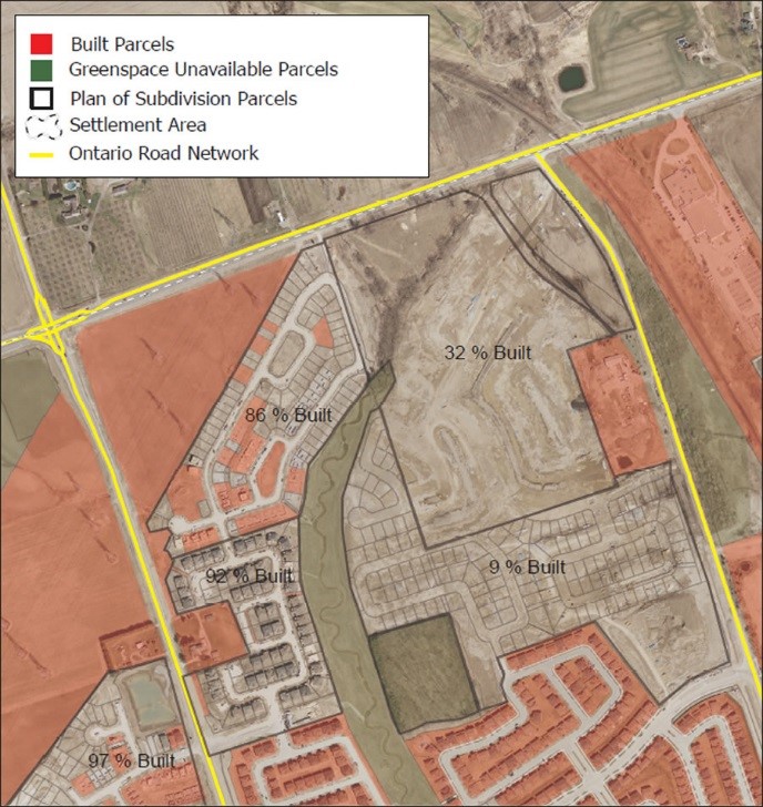
Figure 16a

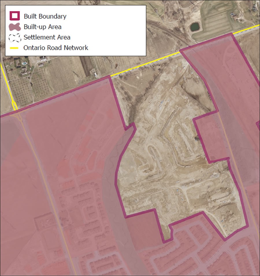
Figure 16b

Rule viii. Align the built boundary with roads, rail lines, and water features

In this rule, the built boundary is generally aligned with centre-lines of roads in the Ontario Road Network (ORN) dataset, active rail lines, or with the edges of water bodies such as rivers and lakes, if such features lie within 100m of either side of the edge of the outermost built parcel.

If the built boundary is aligned with a road which is a 400-series provincial highway, a canal or waterway, or an active rail line, then the edge of the highway adjacent to the built-up area or highway interchange right-of-way, canal right-of-way, or the active rail right-of-way respectively, is the edge of the built-up area.

Figures 17a and 17b illustrate the application of this refinement rule.

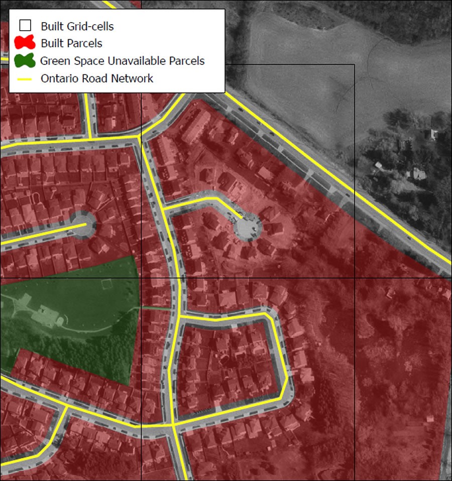
Figure 17a

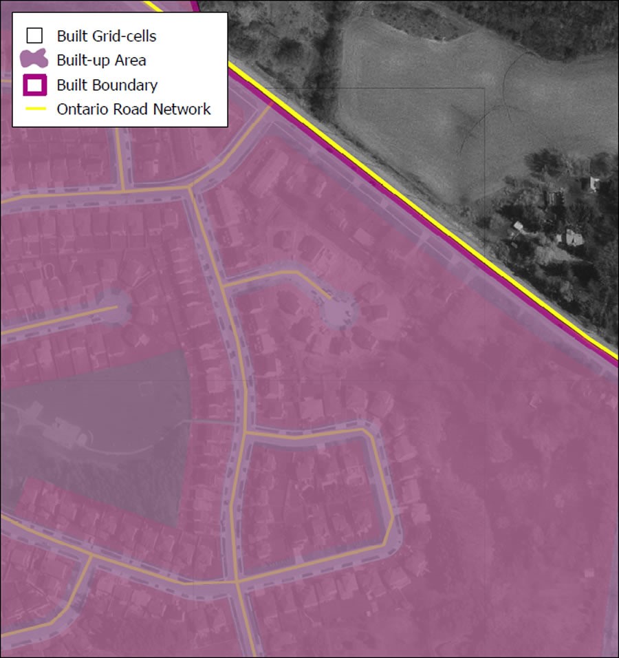
Figure 17b

Figure 17a shows roads within 100m of built parcels. Figure 17b shows the built boundary is established as the centre-line of the road.

Rule ix. Align the built boundary with parcel edges if no appropriate roads or water features are present

If no roads or water features lie within 100m of the edge of the built parcels, the built boundary is aligned with the edge of the outermost built parcel within the settlement area. Figures 18a and 18b below illustrate the application of this refinement rule.

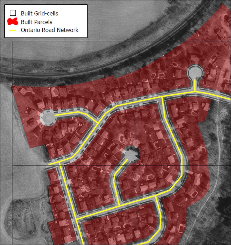
Figure 18a

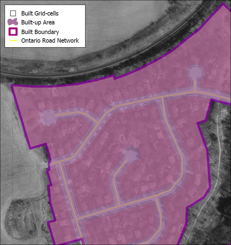
Figure 18b

Figure 18a shows built parcels. Figure 18b shows that the parcel boundary serves as the built boundary in the situation where there is no road or water feature within 100m to align with.

Rule x. Treatment of holes in the built-up area

In order to create a largely contiguous built-up area, groups of unbuilt parcels of less than 37.5 hectares^{footnote 7[7]} and completely surrounded on all sides by built parcels, are included within the built boundary. All urban growth centres are included within the built boundary. Larger vacant areas, greater than 37.5 hectares, remain as greenfield "holes" within the built boundary. In a very limited number of instances, some smaller holes also remain where a municipality considers these areas to be a greenfield rather than built-up area

Figures 19a and 19b below illustrate the application of this refinement rule.

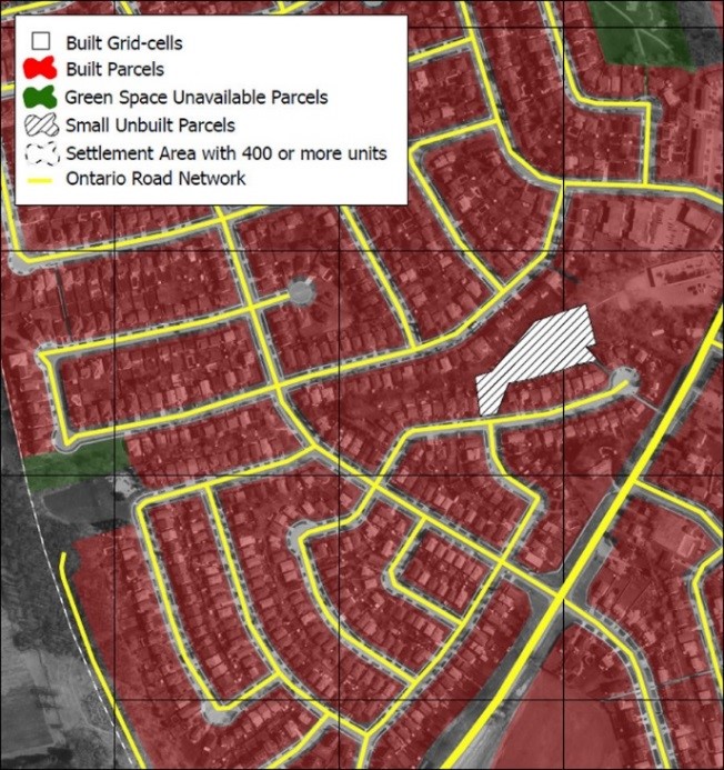
Figure 19a 

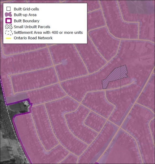
Figure 19b

Figure 19a shows unbuilt areas less than 37.5 hectares surrounded by built areas. Figure 19b shows the built boundary which includes unbuilt areas.

Rule xi. Limit the built boundary to the settlement area boundary

The built boundary must lie within a municipal settlement area boundary. On the ground, individual built parcels may extend beyond settlement area boundaries. In such circumstances those parcels are excluded from the built boundary. Generally, the built boundary follows road centre-lines, water feature edges, and property parcel boundaries, and not the settlement area boundary.

Where the settlement area is defined conceptually in a municipal official plan, and not as an identifiable line, the Ministry of Public Infrastructure Renewal has worked with the municipality to limit the built boundary to within the approximate extent of the settlement area.