Part 3: Scientific principles relevant to this review
Determining causation in the context of workers’ compensation is a complex process primarily governed by legal principles (19), but, hopefully, informed by scientific principles as well. There are a number of national and international agencies and organizations that assess whether chemicals, forms of radiation, or other factors cause cancer. The most widely recognized of these internationally, and in Canada, is IARC, which classifies agents into four categories: Group 1 (definite human carcinogens), Group 2A (probable), Group 2B (possible) and Group 3 (not classifiable) (21,22). IARC's evaluation process, which is well documented, is based on scientific principles and the use of peer-reviewed – and publicly available – scientific evidence.
To do its evaluations, IARC Working Groups conduct reviews of all available human studies. Epidemiologic studies are reviewed using a weight-of-evidence
approach where the results of all studies meeting the minimum quality criteria are considered, rather than focusing on the results of positive studies alone. IARC also evaluates animal and other experimental studies (but uses a different set of pre-defined rules) and has attempted to systematize their approach to identifying and classifying the mechanisms of carcinogenesis (23). In the context of compensation, it is important to recognize that IARC assesses whether a chemical or other agent can cause cancer (a hazard assessment), as opposed to the level of exposure necessary to cause cancer (a risk assessment). There are other organizations (such as the US National Toxicology Program, the US Environmental Protection Agency and the Dutch Expert Committee on Occupational Hazards) that use independent scientific committees to evaluate studies across disciplines
Over the last decade, IARC re-evaluated all Group 1 carcinogens and changed its evaluation process to systematically identify which cancer types (i.e., lung, skin, etc.) are caused by specific carcinogens. This, in my opinion, is a valuable gift to the adjudication process
Multi-stage theory of carcinogenesis
The multi-stage theory of how cancer is caused (also known as the Armitage-Doll model) was developed in 1954 (24). Although other models have been proposed since that time, the basic theory has been well accepted and supported by experimental data. From a practical point of view, these models have contributed to our understanding that a cancer in an individual does not have a single cause but is the result of a complex series of events that occur at different stages, from the initiation of disease
Carcinogens (chemicals, radiation or viruses) can have an impact through various mechanisms at any or multiple stages, from the earliest stages continuing even after the clinical disease has developed (25). Figure 4 below is one representation of how our understanding has continued to increase in sophistication. In the model, there are many stages in the development of cancer, but the earliest stage is still the mutation that results in the initiated cell, while the last potential stage is the development of metastases.
Figure 4: Our evolving understanding of the mechanism of carcinogenesis
See paper on chemical carcinogenesis by Hofseth LJ, Weston A, Harris CC. Chemical carcinogenesis. 2017. [Available from: Oncohema Key].
Latency and induction
Multi-stage theories also relate directly to the concepts of induction and latency. The induction period is when an exposure has its effect on increasing the risk of cancer. Latency refers to the time period between the induction period and the detection of disease. While induction and latency are sometimes treated as a property of a disease, they are actually a property of the relationship between each exposure and the disease (Figure 5). The series of events needed for the development of cancer means that different causes could have different effective time periods of exposure, depending on whether they have early or late stage effects. Thus, there could be differences in the time between when a contributing exposure occurs and the detection of disease.
Figure 5: Latent and induction periods in the chronic disease model
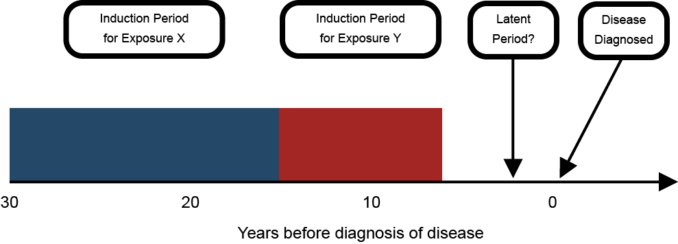
Some epidemiological studies are better suited to assisting with attribution than others. For example, while many studies assume a 10- to 15-year latency lag for asbestos exposure and lung cancer, some researchers have investigated the association between occupational asbestos exposure and lung cancer using a latency modeling approach that allowed the authors to investigate the time since each yearly exposure compared to the time since first exposure. They found that there was a shorter latency period than previously assumed, especially for high intensity of exposure
(26). This study is a powerful illustration of how assuming a default latent period disregards the effect of time and intensity of exposure on the latent period variability.
The role of multiple exposures
Another useful theory of how multiple exposures can contribute is Rothman's causal pie model (27). In this conceptual model, a sufficient cause
of disease is illustrated as a pie consisting of a set of component causes (illustrated as pieces of the pie) that together can cause a disease. An important concept is that sufficient cause
requires all components to operate and if any component is removed, it is no longer sufficient. The causal pie model is illustrated in Figure 6, below, using the example of asbestos exposure, cigarette smoking and lung cancer. In this example, there are three sufficient causes (represented by I, II and III). Sufficient Cause I is asbestos plus some unknown factor or factors, Sufficient Cause II is smoking plus some unknown factor(s), and Sufficient Cause III is asbestos and smoking plus some unknown factor(s). Note that in this example the size of the pie slices does not reflect their relative importance.
Figure 6: Causal pie model – the example of asbestos, smoking and lung cancer*
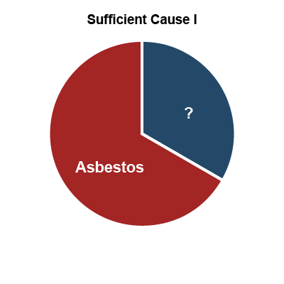
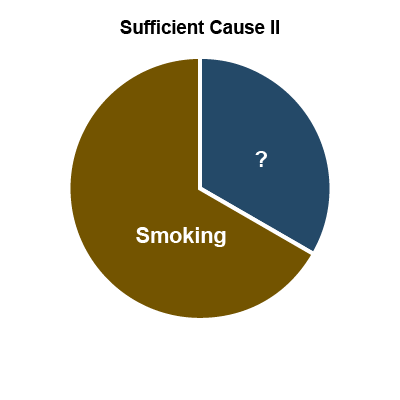
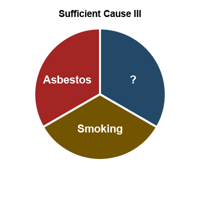
*Rothman’s causal pie model conceptualizes how multiple exposures can contribute to the onset of work-related disease and the sizes of the slices have nothing to do with the relative contributions of each exposure.
The combined impact of multiple causes
The impact of an individual cause can be measured in several ways:
- Added Risk: The first, and perhaps simplest, way to measure the impact of a cause is to consider how much it adds to the risk of disease. For example, if the risk of disease for people who are not exposed to the cause is 2 per 100,000 people, and the risk among people who are exposed is 8 per 100,000 then the added risk is 6 per 100,000.
- Relative Risk: Another way to measure the impact of a cause is to look at the ratio of the risk among those who are exposed vs. those who are unexposed. So, in the above example, the relative risk among exposed people is 4 times the risk of people who are not exposed (i.e., 8 divided by 2).
While there are situations in which individuals are exposed to a single causative agent, it is much more common for people to be exposed to multiple established or suspected human carcinogens at the same time. In these situations, it is also necessary to consider whether the causes act independently or interdependently (i.e., whether they interact with each other).
- Independent causes: Two or more causes are independent if
the occurrence of one is in no way predictable from the occurrence of the other
and the causes do not interact with each other to increase or decrease the risk (28). In this situation, we would generally expect that the combined effect of two or more independent causes would be the sum of their solitary effects. In other words, they have what is called an additive relationship. So, if the risk of chemical X is 6 per 100,000 and the risk of chemical Y is 4 per 100,000, we would expect the risk of cancer to be 10 per 100,000 (i.e., 6+4=10). - Interdependent causes: Two or more causes are interdependent (or interactive) if they operate together to
produce or prevent an effect
(28). In this situation, we would generally expect that the combined effect of two or more interdependent causes would be greater than the sum of their solitary effects. In other words, they have what is called a synergistic relationshipfootnote 13 . So, in the above example, if the two causes interact with each other and create a risk that is greater than 10, we would say there is synergy between the two causes. If the risk in people exposed to both causes were equal to 24 per 100,000, we would say that the relationship is multiplicative (i.e., 6x4=24).
The multistage model predicts that the interaction between two carcinogens acting at different stages can range from purely additive to many times more than multiplicative depending on the sequence and interval between the two exposures
(29,30).
Epidemiologic studies can be used to illustrate some of the principles above. The classic example of interaction is from the 1979 study of New Jersey insulation workers (31). Table 5 presents the reported risks of lung cancer among workers with different exposure histories.
| History of smoking | History of asbestos exposure | Lung cancer mortality rate (per 100,000) | Relative risk of lung cancer |
|---|---|---|---|
| No | No | 11 | Reference |
| No | Yes | 58 | 5.3 |
| Yes | No | 123 | 11.2 |
| Yes | Yes | 602 | 54.7 |
As the table illustrates, the risk associated with exposure to smoking and asbestos is much greater than the sum of the individual risks, indicating an interaction between the two exposures. Because the observed relative risk (54.7) is approximately the same as multiplying the risk among workers only exposed to asbestos (5.3) times the risk among workers who only smoked (11.2), the relationship between smoking and asbestos in this example shows the classic multiplicative relationship (i.e., 5.3 x 11.2 = 59.4). If the exposure to asbestos and smoking had no interaction, then they may have shown an additive relationship (i.e., 5.3 + 11.2 = 16.5), still substantial but much smaller than 54.7. A more important point is that removing asbestos would not only prevent the cancers caused by asbestos alone, but also the cancers caused by the combination of smoking and asbestos, reducing the lung cancer rate in that group to the rate for smokers alone.
While there are too few studies of multiple exposures to quantify the relationship between many of the common workplace exposures, it would seem reasonable to assume in the absence of contrary evidence that they are independent and that therefore their relationship would be assumed to be additive. Such an approach has been taken by the ACGIH® for calculating the Threshold Limit Value for Mixtures for over 30 years (32):
When two or more hazardous substances have a similar toxicologic effect on the same organ or system, their combined effects, rather than that of either individually, should be given primary consideration. In the absence of information to the contrary, different substances should be considered as additive where the health effect and target organ or system are the same.
Appendix E of 2019 TLVs and BEIs(32).
This approach has been adopted in the context of prevention by regulatory agencies within Canada, including WorkSafeBC
Statistical distribution of effects
The final scientific principle that deserves discussion in this area of the report is the statistical distribution of effects. Biological processes, such as the development of disease, generally have what is termed a normal distribution (a bell-shaped curve). For practical purposes, we generally use a discrete range of years or other units when assessing the length or timing of exposure or its latency. For example, we might say that 20 years of exposure
was needed at least 10 years prior to diagnosis
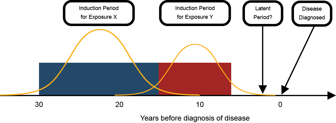
. These numbers are based on epidemiologic studies and represent the period when there was the highest probability that exposure resulted in disease (i.e., the middle portion of the bell-shaped curve). In addition, researchers find round numbers (like 5, 10, 20…) convenient, but biological relationships do not necessarily favour these cut-points. Discrete time ranges for exposure and latency are useful, but it should be recognized that these ranges will not apply to all individuals. The period of time when exposure can contribute to the development of disease is determined by a complex set of factors and some individuals will be in the tail ends of the distribution, outside of the discrete range estimated by epidemiologic studies (Figure 7).
Figure 7: Induction and latency model with statistical distributions overlaid
Footnotes
- footnote[8] Back to paragraph Such as toxicology, occupational hygiene, occupational medicine, and occupational epidemiology.
- footnote[9] Back to paragraph The List of Classifications by cancer sites with sufficient or limited evidence in humans, Volumes 1 to 123 is available from IARC.
- footnote[10] Back to paragraph The first stage of carcinogenesis. The primary step of tumor induction, where the potential for unregulated growth is established.
- footnote[11] Back to paragraph The second stage of carcinogenesis, in which a promoting agent induces an initiated cell to divide abnormally.
- footnote[12] Back to paragraph The third stage of carcinogenesis. A phase of unregulated growth and invasiveness, frequently with metastases and morphologic changes in the cancer cells.
- footnote[13] Back to paragraph It is possible for the combined effect of two or more causes to be less than the sum of their solitary effects (i.e., they combine to create a protective or preventive effect). In this case, the causes have an antagonistic relationship.
- footnote[14] Back to paragraph Section 5.51 of the Occupational Health and Safety Regulation states: If there is exposure to a mixture of 2 or more substances with established exposure limits which exhibit similar toxicological effects, the effects of such exposure must be considered additive unless it is known otherwise, and the additive exposure must not exceed 100%. According to the corresponding guideline, this section applies to all exposure limits, except for excursion limits. The guideline goes on to specify that when considering additive effects, similar exposure limits must be compared and for effects to be considered additive, the substances must act upon the same target organ or target organ system and have similar toxicological effects.