The content on this page is no longer up to date. It will remain on ontario.ca for a limited time before it moves to the Archives of Ontario.
Fuels system 20-year outlook
2.1 Demand Outlook
The demand for fuels is the starting point used in assessing the outlook for fuels in Ontario. There is considerable uncertainty with all demand outlooks, as future demand for fuels will depend on global macroeconomic and fuels market trends and technology development, as well as more local provincial economic, demographic and policy trends.
In preparing this report and the associated analysis, Navigant has considered a range of possible fuels sector characterizations and outlooks for demand, ranging from 1,800 PJ to 2,400 PJ in 2035
The outlooks all reflect actions identified in the government’s recently announced Climate Change Action Plan. The outlooks are all consistent with the outlooks presented by IESO in its OPO, and were developed based on a common set of assumptions and data regarding economic activity, demographics, fuel shares, electrification, pricing, weather, etc.
Figure 27: Demand Uncertainty
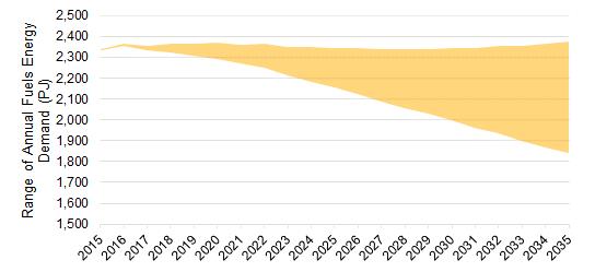
Accessible data table for Figure 27
Source: CanESS, 2016
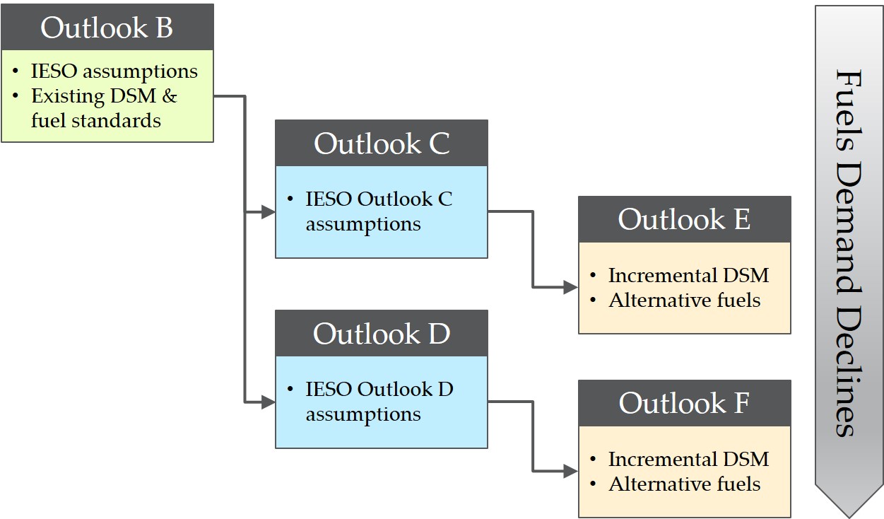
The outlooks considered for Ontario’s energy fuels demand are:
- Outlook B, which reflects all of the assumptions adopted by IESO for the OPO Outlook B, and further assumes that natural gas demand-side management (DSM) programs supporting efficiency and conservation improvements will continue at present levels of funding and that transportation fuels standards will proceed as planned.
- Outlooks C and D, which reflect all of the assumptions adopted by IESO for the OPO Outlooks C and D, and further assume that natural gas DSM will continue at present levels of funding and that transportation fuels standards will proceed as planned.
- Outlooks E and F, which reflect all of the assumptions adopted by IESO for the OPO Outlooks C and D (respectively), but also explore different levels of additional natural gas DSM, and the displacement of some conventional fuels with less carbon-intense alternatives.
Outlook A was developed by IESO to explore the implications of lower electricity demand. Applying the assumptions of Outlook A to the fuels sector would result in lower fuels demand than Outlook B. Lower fuels demand is already explored in the FTR by Outlooks C, D, E and F. Given the time constraints under which the FTR was developed, and the fact that lower fuels demand scenarios were already being explored by four alternative outlooks, it was determined that modeling Outlook A would provide incremental information of only limited value. Outlook A has therefore not been modeled as part of the FTR.
The incremental relationships between these outlooks, and their relative position in the range of fuels energy demand highlighted in Figure 27, above, is illustrated in Figure 28, below.
Figure 28: Illustration of Outlook Relationships
The total energy-related fuels demand of each outlook is illustrated in Figure 29, below. As may be seen, in the final year of the outlook horizon, Outlook F yields a total Ontario energy-related fuels demand that is 23% lower than that projected by Outlook B.
Figure 29: Five Fuels Energy Demand Outlooks
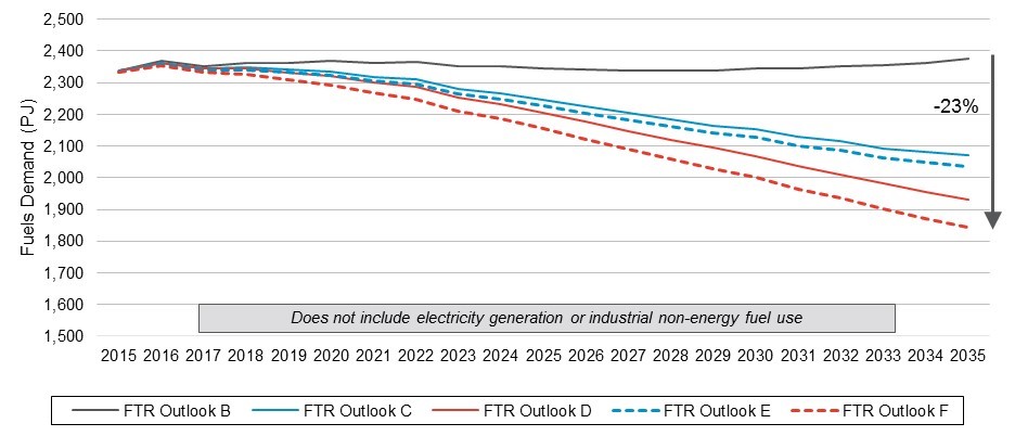 Accessible data table for Figure 29
Source: CanESS & Navigant Analysis, 2016
The fuels energy demand in 2035 (as well as the initial 2015 levels) by sector across the five outlooks is illustrated in Figure 30, below. The majority of fuels energy in all outlooks is consumed by the industrial and transportation sectors, which together account for approximately three-quarters of total fuels energy demand.
Figure 30: Sectoral Breakdown of Energy Demand by Outlook, 2015 vs 2035
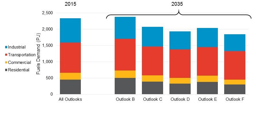
Accessible data table for Figure 30
Source: CanESS & Navigant Analysis, 2016
Assumptions across the demand outlooks are summarized in Table 1, below. The following acronyms appear in this table:
- EV: electric vehicles
- DSM: demand-side management (natural gas focused conservation)
- OEB: Ontario Energy Board
- APS: Achievable Potential Study, the OEB’s Natural Gas Conservation Potential Study
footnote 13 - RNG: Renewable natural gas
- CNG: Compressed natural gas
- LNG: Liquefied natural gas
| Sector | Outlook B | Outlook C | Outlook D | Outlook E | Outlook F |
|---|---|---|---|---|---|
| Residential | 498 PJ in 2035 | Oil and propane heating switches to heat pumps, electric and water heating gain 25% of gas market share. (388 PJ in 2035) | Oil and propane heating switches to heat pumps, electric and water heating gain 50% of gas market share. (322 PJ in 2035) | Assumptions as per Outlook C, plus:
(381 PJ in 2035) | Assumptions as per Outlook D, plus:
(302 PJ in 2035) |
| Commercial | 233 PJ in 2035 | Oil and propane heating switches to heat pumps, electric and water heating gain 25% of gas market share. (192 PJ in 2035) | Oil and propane heating switches to heat pumps, electric and water heating gain 50% of gas market share. (177 PJ in 2035) | Assumptions as per Outlook C, plus:
(187 PJ in 2035) | Assumptions as per Outlook D, plus:
(147 PJ in 2035) |
| Industrial | 671 PJ in 2035 | 5% of 2012 fossil energy switches to electric equivalent (607PJ in 2035) | 10% of 2012 fossil energy switches to electric equivalent (550 PJ in 2035) | Assumptions as per Outlook C, plus:
(591 PJ in 2035) | Assumptions as per Outlook D, plus:
(519 PJ in 2035) |
| Transportation | 967 PJ in 2035 |
(883 PJ in 2035) |
(883 PJ in 2035) | Assumptions as per Outlook C, plus:
(878 PJ in 2035) | Assumptions as per Outlook D, plus:
(874 PJ in 2035) |
| Total | 2,377 PJ in 2035 | 2,070 PJ in 2035 | 1,931 PJ in 2035 | 2,037 PJ in 2035 | 1,842 PJ in 2035 |
Each of the following sub-sections illustrate changes in fuel demand over time for each sector (residential, commercial, industrial, transportation). Each chart shows a single sector, and compares fuels use in 2025 and in 2035 to fuels use in 2015 by fuel for three outlooks: B, D and F.
The purpose of this sectoral breakdown is to contrast IESO outlooks (C and D) with those that assume incremental natural gas DSM and additional use of alternative fuels (E and F). Since C and D (and E and F) differ from each other only in degree, only the most extreme outlooks from the two groups (i.e., D and F) are shown.
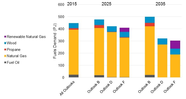
2.1.1 Residential
Outlook D results in a substantial reduction in residential fuels demand (relative to Outlook B) as a result of IESO assumptions regarding the electrification of space and water heating. Total residential fuel demand in 2035 is 35% lower in Outlook D than it is in Outlook B. Total residential energy use in 2035 in Outlook F is four percentage points lower than in Outlook D (or 39% less than in Outlook B) as a result of incremental natural gas DSM. In addition to this, however, a substantial volume of conventional natural gas (66 PJ) has been replaced by renewable natural gas (RNG).
Residential fuels energy demand for Outlooks B, D and F in 2025 and 2035 are illustrated in Figure 31 below.
Figure 31: Residential Outlook
Accessible data table for Figure 31
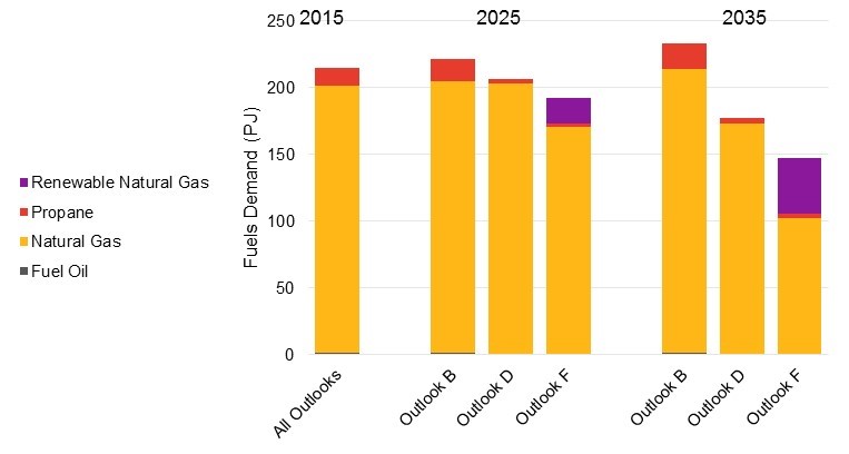
2.1.2 Commercial
Outlook D results in a substantial reduction in commercial fuels demand (relative to Outlook B) as a result of IESO assumptions regarding the electrification of space and water heating. Total commercial fuel demand in 2035 is 24% lower in Outlook D than it is in Outlook B. Total commercial energy use in 2035 in Outlook F is thirteen percentage points lower than in Outlook D (or 37% less than in Outlook B) as a result of incremental natural gas DSM. In addition to this, however, a substantial volume of conventional natural gas (42 PJ) has been replaced by renewable natural gas (RNG).
Commercial fuels energy demand for Outlooks B, D, and F in 2025 and 2035 are illustrated in Figure 32 below.
Figure 32: Commercial Outlook
Accessible data table for Figure 32
Source: CanESS & Navigant Analysis, 2016
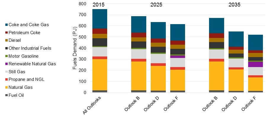
2.1.3 Industrial
Outlook D results in a substantial reduction in industrial fuels demand (relative to Outlook B) as a result of IESO assumptions regarding the electrification of industrial processes. Total industrial fuel demand (for energy use) in 2035 is 18% lower in Outlook D than it is in Outlook B. Although smaller, as a proportion of total sectoral fuels energy use, than the reduction observed in the residential and commercial sector, the total energy reduction in the industrial sector in Outlook D (compared to Outlook B) by 2035 is more than twice the commercial energy reduction.
Total industrial energy use in 2035 in Outlook F (excluding non-energy fuels use) is approximately five percentage points lower than in Outlook D (or 23% less than in Outlook B) as a result of incremental natural gas DSM. In addition to this, however, a substantial volume of conventional natural gas (48 PJ) has been replaced by renewable natural gas (RNG).
Industrial fuels energy demand for Outlooks B, D and F in 2025 and 2035 are illustrated in Figure 33 below.
Figure 33: Industrial Outlook
Accessible data table for Figure 33
Source: CanESS & Navigant Analysis, 2016
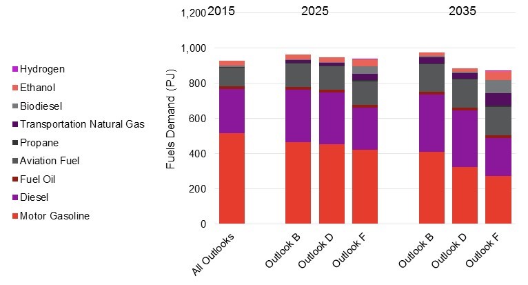
2.1.4 Transportation
Outlook D results in a moderate reduction in transportation fuels demand (relative to Outlook B) as a result of IESO assumptions regarding the adoption of EVs. Total transportation fuel demand in 2035 is 9.5% lower in Outlook D than it is in Outlook B. As in the case of the industrial sector, this reduction, although small in proportion to total transportation fuels use, is substantial in absolute terms – 92 PJ, compared to Outlook B, nearly twice the energy reduction observed in the commercial sector in Outlook D relative to Outlook B.
Total energy use in 2035 in Outlook F is less than one percentage point lower than in Outlook D (or 10.4% less than in Outlook B). This is due to the fact that the transportation sector assumptions for Outlook F (incremental to Outlook D) are all related to fuel switching. Some modest energy reductions are observed due to improved efficiencies associated with some technologies and fuels, but since incremental Outlook F assumptions are based on a movement toward fuels with lower GHG emissions, little change is seen in total energy consumption.
The most substantial fuel switching impacts observed in Outlook F are those associated with ethanol (for light duty vehicles), bio-based diesels and natural gas (for heavy duty vehicles). Outlook F also considers the impact of increased use of hydrogen fuel cell vehicles (HFCV) and propane-fueled vehicles, but the impact of these changes is more modest.
Transportation fuels energy demand for Outlooks B, D and F in 2025 and 2035 are illustrated in Figure 34 below.
Figure 34: Transportation Outlook
Accessible data table for Figure 34
Source: CanESS & Navigant Analysis, 2016
2.2 Conservation Outlook
Conservation potential is a key component of IESO’s outlooks for the Ontario electricity system, and is embedded in all of the outlooks modeled in the OPO. This conservation is achieved through the deployment of conservation programs targeting different end-uses across different sectors, as well as municipal, provincial and federal codes and standards.
For most of the fuels sector, no corresponding portfolio of conservation programs exists, with the exception of natural gas DSM programs from the regulated natural gas utilities. Other specific conservation initiatives in the fuels sector include codes and standards relating to new equipment and construction, and vehicle fuel economy standards.
Outlooks B, C and D all reflect the assumption that natural gas DSM programs will continue at current (i.e., 2017 – 2020) levels of funding. The natural gas DSM in each of these outlooks approximately corresponds to the “constrained achievable” potential mapped out in the Ontario Energy Board’s Conservation Potential study.
Codes and standards affecting natural gas consumption are not included in the OEB study and are not explicitly modeled in CanESS in the same way that vehicle fuel economy standards are. The effects of building codes and other types of standards affecting residential, commercial and industrial natural gas use are captured through the extension forward of declining trends in energy intensity in those sectors.
All of the FTR outlooks also reflect fuels standards regulation currently in force, and the more stringent fuel economy standards scheduled to come into effect in the future. These standards include both U.S. Environmental Protection Agency (EPA)
- The Corporate Average Fuel Economy (CAFE) standard. This applies to cars and light trucks.
- The Fuel Efficiency and GHG Emission Program for Medium- and Heavy-Duty Trucks. This applies to medium and heavy-duty trucks.
The conservation impact of vehicle codes and standards natural gas DSM is illustrated in Figure 35 below. A more detailed breakdown of the composition of natural gas DSM potential through to 2030 (e.g., by end-use, sector, etc.) may be found in the OEB report cited above.
Figure 35: Conservation Achievement and Outlook to 2035 (Outlook B)
Accessible data table for Figure 35
Source: CanESS & Navigant Analysis, 2016
2.3 Supply Outlook
As discussed, fuels are supplied by a series of robust commodity markets where the demand for product is essential in establishing supply, infrastructure and processing needs. Fuels markets are flexible, responsive to demand shifts and price changes. Supply infrastructure is also typically responsive to changes in demand, which provides a strong signal for investment needs. In all scenarios, the supply outlook is expected to provide sufficient quantities of product to meet Ontario’s demands for conventional fossil fuels. Current and planned infrastructure could be capable of meeting the demands in Outlook B, which is based on a relatively flat demand for fossil fuels, as well as all other Outlooks where fossil fuel demand is contracting. Assuming the appropriate contribution of reinvestments and proper maintenance to processing, storage, transmission and distribution facilities, no issues in supply are projected.
Where outlooks see demand growth for alternative fuels, new investment in infrastructure and greater expectations for imports of alternative fuels will be required. New ethanol processing facilities and biodiesel refineries may be needed in outlooks with higher demands for alternative fuels, along with the associated investment in storage, distribution networks and terminal asset.
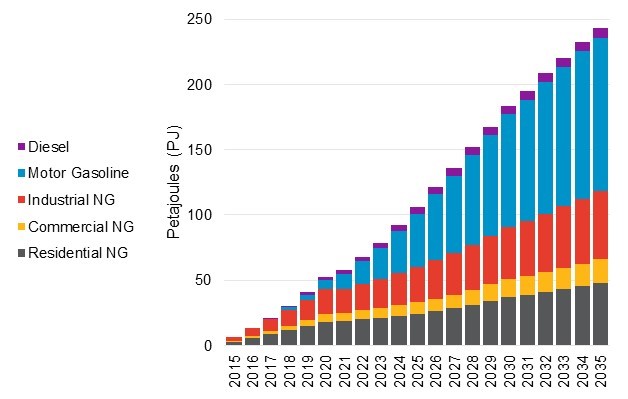
Figure 36 below, below, illustrates the range of demands that supply systems could need to meet by 2035 as conditions in the market change. Existing infrastructure for conventional fossil fuels is likely to be sufficient, while the substantial change across outlooks in alternatives will require new investments in processing and delivery infrastructure.
Figure 36: Alternative Fuels in 2035 – Outlook B and F
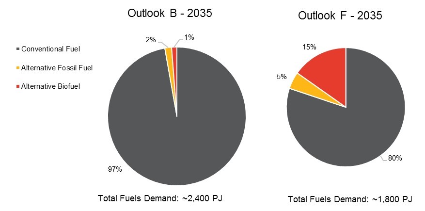
Accessible data table for Figure 36
Source: CanESS & Navigant Analysis, 2016
A more detailed breakdown of the composition of alternative fuels in Outlook F, and how that changes over time, is shown in Figure 37, below.
Figure 37: Outlook F Alternative Fuel Breakdown
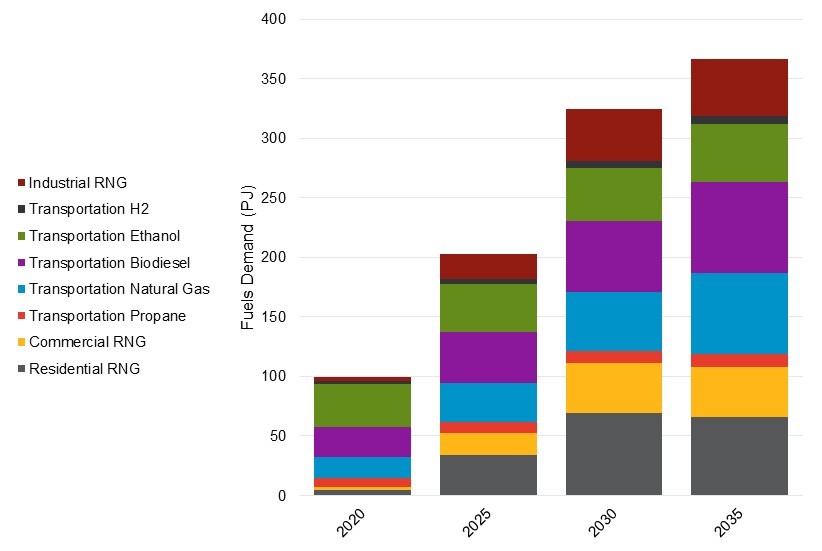
Accessible data table for Figure 37
Source: CanESS & Navigant Analysis, 2016
At present, limited renewable natural gas facilities exist in Ontario, and production capacity at these facilities would be insufficient to satisfy the requirements of either Outlook E or Outlook F. Likewise, bio-based diesel refineries in Ontario have a total production capacity of approximately 300 million litres per year
Development of domestic biofuel production capacity, or the sourcing of substantial volumes of imports would be required to meet the biofuels demands of Outlook F.
2.3.1 Supply Resources
Ontario’s non-electric energy needs have historically been satisfied by a wide variety of fuels. The diverse nature of the fuels sector is a function of both free-market dynamics, and the diverse requirements and niche needs of Ontario’s fuel users. No single fuel is suitable for all applications. The characteristics of the major groups of fuels considered in this report are discussed below.
2.3.1.1 Conservation Conservation is not in itself a fuel, but can be used as way of reducing fuel consumption. As noted in the Conservation Outlook, aside from natural gas, program-driven energy conservation does not generally exist in the fuels sector. The potential for natural gas DSM (conservation), based on the findings of the OEB’s Conservation Potential Study, have been accounted for in all five outlooks, as have fuel economy standards.
2.3.1.2 Natural gas Natural gas is the most common heating fuel in Ontario, by share. However, natural gas is not accessible to all Ontario consumers because the distribution network is not available to all regions. Generally, rural or remote parts of the province are not served by natural gas piping networks. Delivery of liquified natural gas and compressed natural gas by truck or rail is a possible alternative. Adoption of this fuel has been encouraged by the gradual expansion of the distribution network, and historically low prices in relation to other space- and water-heating fuel options. Most of Ontario’s natural gas is currently transported to the province via pipeline from Western Canada
2.3.1.3 Renewable natural gas Renewable natural gas (RNG) is a biogas product of the decomposition of organic matter. Biogas can be derived from landfills, livestock operations, wastewater treatment, or waste from industrial, institutional, and commercial entities. As outlined in a 2014 CanBio Report entitled Status on Bioenergy in Canada,
2.3.1.4 Propane Propane is a stable, economically transportable alternative to natural gas and is used for space-heating in remote areas without access to natural gas, for transportation and in industrial applications. Propane’s stability and storage longevity contribute to its adoption by remote communities and industry. Historically propane was produced using oil by-products (liquefied petroleum gas), but currently the majority of Ontario’s propane supply is derived from natural gas (natural gas liquid) produced in Alberta.
2.3.1.5 Oil products Refined oil products are used principally as a transportation fuel (gasoline, diesel, aviation fuel). Fuel oil is also used for industrial process heating and home heating, although home heating use of fuel oil has been in decline for some time, due partly to the high cost of the product and to the insurance premiums required of homeowners that use oil. Although a very modest amount of crude oil is produced in Ontario, the majority of Ontario’s oil products are refined in Ontario using crude oil transported from Alberta.
2.3.1.6 Ethanol Despite Ontario producing more bioethanol than any other province in Ontario, the province imports approximately 20% of its current requirements.
2.3.1.7 Biodiesel There are two types of bio-based diesel: “biodiesel”, and “renewable” diesel. The key difference between the two is that biodiesel congeals at higher temperatures than petro-diesel limiting the blend rate for this fuel in colder months. Renewable diesel does not have this limitation and may be blended (or used without blending) in all conditions suitable to petro-diesel. Ontario biodiesel refineries (including one not yet operational) have a nominal production capacity of nearly 300 million litres a year, equivalent to approximately 10 PJ.
2.3.1.8 Hydrogen Hydrogen is considered in this report only as a fuel for hydrogen fuel cell vehicles (HFCVs). Currently, most hydrogen is produced from methane or coal gasification, although some is also produced via the gasification of biomass or water electrolysis. Hydrogen may be produced without carbon emissions by using electrolysis with electricity from non-emitting sources. There are currently two hydrogen production facilities in Ontario, both in Sarnia, with a total production capacity of 230,000 kg per day, equivalent to approximately 10 PJ per year.
2.4 Emissions Outlook
Carbon emissions from Ontario’s fuels sector are projected to decline significantly under Outlooks C, D, E and F. Emissions reductions observed in Outlooks C and D are driven mainly by the electrification assumed to take place across all sectors. Further emissions reductions identified through Outlooks E and F are the result of incremental natural gas DSM and to the increased use of alternative, less carbon-emitting fuels.
Outlook F delivers the most substantial emissions reductions, relative to 2014, with 46 MT of annual reductions by 2035.
GHG emissions that result from energy related fuels use across the outlooks are illustrated in Figure 38 below. This includes only combustion-related fuels emissions and does not include emissions from electricity generation fuels use, which are addressed within the OPO. Outlook F (combining both electrification initiatives and fuels-directed initiatives) yields substantial decarbonisation potential, reducing emissions of CO2e by nearly 40% in 2035 compared to Outlook B. Figure 38: Fuels Combustion GHG Emissions Outlook 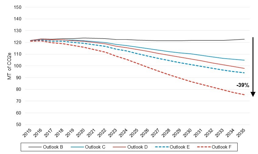 Accessible data table for Figure 38
Source: CanESS & Navigant Analysis, 2016
The majority of emissions reductions in Outlooks C through F are realized in the industrial and transportation sectors. Although energy reductions in these sectors across the outlooks are less than those observed for the residential sector, emissions potential is greater due to more carbon-intensive nature of the fuels used for energy in those sectors. The difference, by sector and outlook between emissions in 2014
Figure 39: Emissions Relative to 2014 Levels
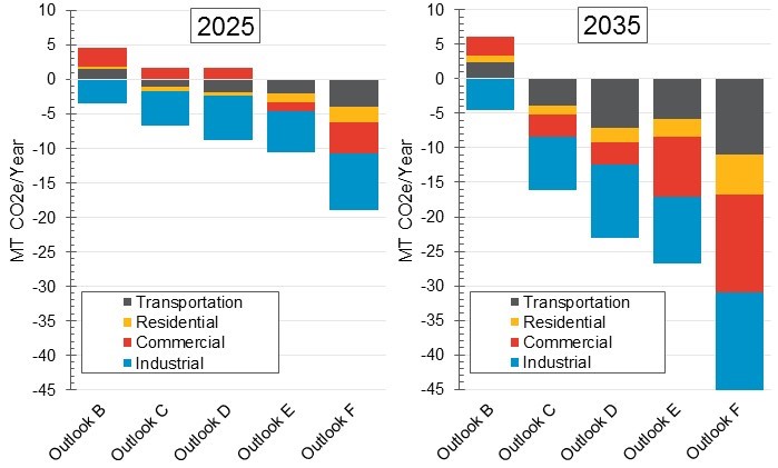
Accessible data table for Figure 39
Source: CanESS & Navigant Analysis, 2016
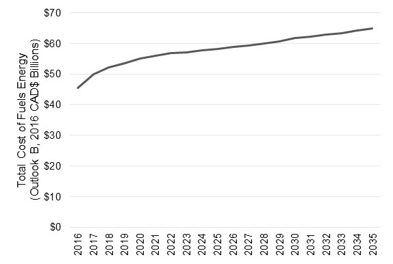
2.5 Fuels System Cost Outlook
The total cost of fuels service over the planning outlooks will be determined by global fuel prices, the mix of fuels demanded (or mandated) in Ontario, the carbon costs of cap and trade, and the costs of maintaining existing regulated natural gas delivery infrastructure. The growth in these costs across the planning horizon is shown in Figure 40, below.
Figure 40: Total Cost of Fuels for Energy in Outlook B
Accessible data table for Figure 40
In Outlook B, the total cost of fuels for energy use would increase by approximately 40%, or about twenty billion dollars between 2016 and 2035. The principal driving factors for this increase in total fuels costs are increasing fossil fuel prices – particularly transportation fuel prices – and the carbon cost of fossil fuel emissions (i.e., the cap and trade carbon price).
The distribution of the increase in system costs for Outlook B is shown in, Figure 41 below.
Figure 41: Drivers of System Cost Increases 2016 to 2035
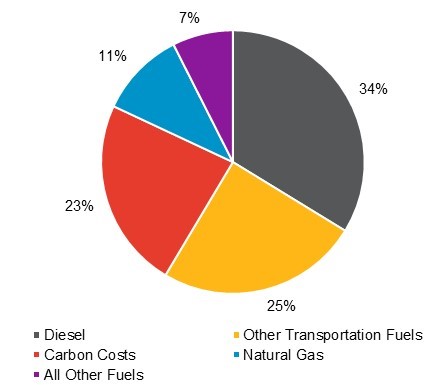
Accessible data table for Figure 41
Source: CanESS & Navigant Analysis, 2016
Approximately one third of the total cost increase is due to the increased use of diesel fuel (up 20% in 2035 from 2016), combined with the increased price of that fuel (up 30% in real terms in 2035 from 2016) under conditions of the outlook. Increasing use of aviation fuel (up 47% from 2016) and the cost of aviation fuel (twice the cost in 2035 as in 2016) is the driver of the increased costs observed for “Other Transportation Fuels”.
Increases in the system cost of natural gas are due almost entirely to changes in the total delivered cost of gas (up 36% from 2016 to 2035) to procure gas supplies and maintain the supply network. Growth in gas consumption is expected to be very modest in Outlook B (up approximately 1% in 2035 from 2016). Although motor gasoline’s unit cost rises by approximately the same ratio as diesel, the impact of this price change on total cost is almost entirely offset by the substantial increase in the use of EVs assumed for this Outlook.
The average unit cost of both natural gas and transportation fuels (inclusive of carbon prices) increases at a decreasing rate for the first few years of the Outlook and then, by 2021, stabilizes at an annual increase of approximately 1% per year. The increase in unit costs are due entirely the forecast increase in the delivered price of these products and the cost of carbon flowing from Ontario’s cap and trade regime.
Figure 42: Average Unit Cost of Natural Gas
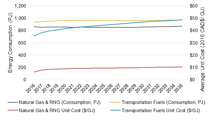
Accessible data table for Figure 42
Source: CanESS & Navigant Analysis, 2016
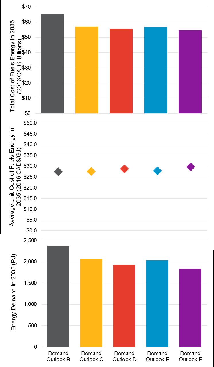
Total fuels energy costs fall substantially in the alternative outlooks, C through F, as may be seen in Figure 43. This is due to a number of factors, principally the reduction in fuel use as a result of electrification of space-heating, industrial processes and light-duty transportation (Outlook C and D). It is these electrification Outlooks that result in the biggest impact to total fuels energy costs. Outlook E and F deliver very modest additional reductions in total fuel cost as a result of incremental natural gas DSM, and the shifting of fuel consumption to less carbon-intensive fuels with commensurately lower carbon costs (Outlook E and F).
Despite total costs falling substantially as a result of electrification, average unit costs increase very modestly across the five outlooks. This is principally the result of the distribution component of natural gas costs, which (different from all other fuels) are assumed to be fixed, regardless of reductions in volume consumed.
Figure 43: Cost of Fuels Energy Across Demand Outlooks
Accessible data table for Figure 43
Source: CanESS & Navigant Analysis, 2016
Footnotes
- footnote[11] Back to paragraph This range includes only fuels used to provide energy. Non-energy fuel use by the industrial sector is not considered in the outlooks.
- footnote[12] Back to paragraph Figures do not include industrial non-energy use fuels demand.
- footnote[13] Back to paragraph ICF International, submitted to the Ontario Energy Board, Final Report: Natural Gas Conservation Potential Study, June 30, 2016, updated July 7, 2016
- footnote[14] Back to paragraph By 2035, of the number of natural gas-fueled space and water heating equipment being sold in Outlook B (due to existing equipment reaching end of life and new additions driven by growth in the residential and commercial sectors), 25 percent of this stock in Outlook C and 50 percent in Outlook D is replaced with air-source heat pumps.
- footnote[15] Back to paragraph ICF International, submitted to the Ontario Energy Board, Final Report: Natural Gas Conservation Potential Study, June 30, 2016, updated July 7, 2016
- footnote[16] Back to paragraph Navigant has worked closely with detailed sectoral and end-use data from the achievable potential study provided by the OEB to calibrate its DSM assumptions, and although the DSM assumed for the FTR is nearly identical at the aggregate level for Outlook B, it varies slightly at the sectoral level. Most, but not all, of this variation at the sectoral level is accounted for by differing sectoral definitions: the OEB report defines multi-family residential as part of the commercial sector, whereas in the FTR this segment falls in the “residential” sector. Likewise, the OEB study includes electricity generation (“utilities”) in the “industrial” sector whereas the FTR does not. Once sectoral definitions are adjusted appropriately some small sectoral differences in total estimated consumption remain, but are extremely low at the aggregate provincial level, for Outlook B.
- footnote[17] Back to paragraph Canadian fuel economy standards are harmonized with U.S. standards.
- footnote[18] Back to paragraph Renewable Industries Canada, Industry Map. Accessed June, 2016.
- footnote[19] Back to paragraph Renewable Industries Canada, Industry Map. Accessed June, 2016.
- footnote[20] Back to paragraph Navigant, North America Natural Gas Market Outlook, Spring 2016
- footnote[21] Back to paragraph Renewable Energies, 2014 Canbio Report on the Status of Bioenergy in Canada. December, 2014.
- footnote[22] Back to paragraph ICF International on behalf of Enbridge Gas Distribution and Union Gas, Results from Aligned Cap & Trade Natural Gas Initiatives Analysis, November 2015 Filed with the Ontario Energy Board: 2016-04-22 EB-2016-0004, Exhibit S3.EGDI.OGA.3
- footnote[23] Back to paragraph National Energy Board and Competition Bureau, Propane Market Review – Final Report, April 2014
- footnote[24] Back to paragraph Statistics Canada, Table 134-0001: Refinery Supply of Crude Oil and Equivalent, Annual
- footnote[25] Back to paragraph Ethanol production data provided by the Ministry of the Environment and Climate Change
- footnote[26] Back to paragraph International Council on Clean Transportation, Technical Barriers to the Consumption of Higher Blends of Ethanol, February 2014
- footnote[27] Back to paragraph Renewable Industries Canada, Industry Map. Accessed June, 2016.
- footnote[28] Back to paragraph Renewable Industries Canada, Industry Map. Accessed June, 2016.
- footnote[29] Back to paragraph Hydrogen Analysis Resource Center, Merchant Hydrogen Plant Capacities in North America, accessed September 2016
- footnote[30] Back to paragraph The anchor year of 2014 (rather than 2015 or 2016) is used for the emissions comparison to allow for comparisons with values included in the 2014 Ontario Climate Change Update, as well as the values reported by Environment Canada (last actuals reported are for 2014) Government of Ontario, Ministry of the Environment and Climate Change, Ontario’s Climate Change Update 2014, 2014
- footnote[31] Back to paragraph Does not include industrial non-energy use natural gas.